Page 117 - Pipelines and Risers

90 Chapter 6

If “N” is the number of wave components, the sea state at a particular time and location can
be represented by:

Surface elevation,
N
q = Eai . sin(oit - k,x +a,) (6.19)
i =I
Velocity component in the x-direction,
a,k, cosh(ki (d + 2))
v,=g.Z -. .sin(-oit -kix+ai) (6.20)
i=l cosh(kid)
Velocity component in the z-direction,
v,=g-c -. .COS(Wit - kix +ai) (6.21)
a, ki sinh( ki (d + 2))
i=l cosh(kid)
Acceleration component in the x-direction,
cosh(ki (d + z))
t -
a, =g-caiki. *COS(O, kix + ai ) (6.22)
i=l cosh(k,d)
Acceleration component in the z-direction,
N sinh( k (d + z))
a, =-g.xaiki‘ sin( o, - kix + ai ) (6.23)
t
i=l cosh( kid)
Dynamical pressure,
cosh(ki (d + z))
PdYn =pg’xai cosh(kid) sin(oi t - kix + ai) (6.24)
i=l

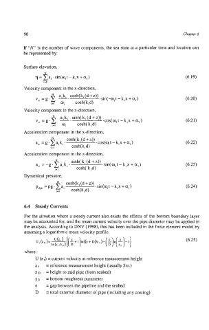
6.4 Steady Currents

For the situation where a steady current also exists the effects of the bottom boundary layer
may be accounted for, and the mean current velocity over the pipe diameter may be applied in
the analysis. According to DNV (I998), this has been included in the finite element model by
assuming a logarithmic mean velocity profile.
(6.25)

where:
U (z = current velocity at reference measurement height
z = reference measurement height (usually 3m.)
z D = height to mid pipe (from seabed)
z 0 = bottom roughness parameter
e = gap between the pipeline and the seabed
D = total external diameter of pipe (including any coating)