Page 67 - Power Electronic Control in Electrical Systems

//SYS21/F:/PEC/REVISES_10-11-01/075065126-CH002.3D ± 57 ± [31±81/51] 17.11.2001 9:49AM

Power electronic control in electrical systems 57

The resulting compensating admittances are given in equation (2.29).
p 
jB gab ˆ jB ab ‡ j(G ca G bc )= 3
p 
jB gbc ˆ jB bc ‡ j(G ab G ca )= 3 (2:29)
p 
jB gca ˆ jB ca ‡ j(G bc G ab )= 3

2.10 Power flow and measurement

2.10.1 Single-phase

Suppose we have a single-phase load as in Figure 2.7 supplied with a sinusoidal
p
voltage whose instantaneous value is u ˆ V m cos ot. The RMS value is V ˆ V m / 2
and the phasor value is V. If the load is linear (i.e. its impedance is constant and does
not depend on the current or voltage), the current will be sinusoidal too. It leads or
lags the voltage by a phase angle f, depending on whether the load is capacitive or
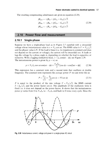
inductive. With a lagging (inductive) load, i ˆ I m cos(ot f); see Figure 2.29.
The instantaneous power is given by p ˆ ui,so

V m I m
p ˆ V m I m cos ot cos(ot f) ˆ [ cos f ‡ cos(2ot f)] (2:30)
2
This expression has a constant term and a second term that oscillates at double
frequency. The constant term represents the average power P: we can write this as

V m I m
P ˆ p p cos f ˆ VI cos f (2:31)

2 2

p
P is equal to the product of the rms voltage V ˆ V m /2, the RMS current
p
I ˆ I m /2, and the power factor cos f. The amplitude of the oscillatory term is
fixed: i.e. it does not depend on the power factor. It shows that the instantaneous
power p varies from 0 to V m I m to V m I m and backto 0 twice every cycle. Since the

Fig. 2.29 Instantaneous current, voltage and power in a single-phase AC circuit.