Page 70 - Power Electronic Control in Electrical Systems

//SYS21/F:/PEC/REVISES_10-11-01/075065126-CH002.3D ± 60 ± [31±81/51] 17.11.2001 9:49AM

60 Power systems engineering ± fundamental concepts

Electronic wattmeter
These instruments multiply the instantaneous voltage and current together and take
the average. Both digital and analog models are available. They are designed to be
used with CTs and VTs, (current transformers and voltage transformers) and they
come in single-phase and three-phase versions. Single-phase instruments have band-
widths up to several hundred kHz, so they give effective readings with distorted
waveforms such as are caused by rectifiers and inverters, provided the harmonic
content is not too great. See Figure 2.32.

Processing of sampled waveforms
The most exacting power measurements are in circuits with high-frequency switching
(as in power electronics with PWM [pulse-width modulation]), especially if the power
factor is low. In these cases the technique is to sample the voltage and current at high
frequency and then digitally compute the power from the voltage and current
samples: u [1, 2, . . . k .... N] and i [1, 2, . . . k .... N]. The average power over time T
is computed from:
N
N
1 X 1 X
P avg ˆ p[k] t ˆ u[k]i[k] t, where T ˆ (N 1) t (2:36)
T T
kˆ1 kˆ1
Some digital processing oscilloscopes can perform this function, but there are spe-
cialist data acquisition systems with fast sampling and analog/digital conversion, and
they may include software for processing the equation (2.36).
The sampling process is illustrated in Figure 2.33. The double samples at the steep
edges in the voltage waveform show the ambiguity (uncertainty) that arises when the
sampling rate is too low relative to the frequency content of the sampled waveform.
This is a particular problem in power electronics, where the voltage may switch from
0±100% in the order of 1 ms. If we use a sampling frequency of 10 MHz to give 10
samples on each voltage switching, then if the fundamental frequency is 50 Hz we will
7
need 1/50 10 ˆ 200 000 samples for just one cycle. This illustrates the tradeoff
between sample length and sampling frequency. The tradeoff is more difficult if a high
resolution is required (for example, 12-bit A/D conversion, a resolution of 1 part in 4096).
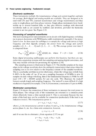
Wattmeter connections
Figure 2.34 shows the connection of three wattmeters to measure the total power in
three phases. The voltage coils of the wattmeters are returned to a common point
which effectively forms a false neutral point 0. This is convenient because the star
point of the load may not be available for connection (particularly if the load is an
induction motor). The instantaneous power is
(2:37)
p ˆ u as i a ‡ u bs i b ‡ u cs i c
where i a is the instantaneous current in phase A and u as is the instantaneous voltage
across phase A, etc. In a three-wire connection, however,
i a ‡ i b ‡ i c ˆ 0 (2:38)
and if we use this to eliminate i c from equation (2.37) we get

p ˆ (u as u cs )i a ‡ (u bs u cs )i b
(2:39)
ˆ u ac i a ‡ u bc i b