Page 553 - Practical Design Ships and Floating Structures

528

For the wind resistance coefficients, the JTTC standard curve and twenty-two Blendermann’s curves
can be selected as an option (Blendermann, 1991). It needs lots of interpolation routines in this
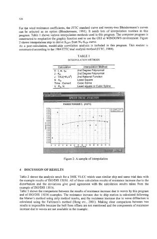
program. Table 1 shows various interpolation methods used in this program. The computer program is
constructed to emphasize the graphic function and to use the GUI at WINDOWS environment. Figure
2 shows interpolation step to derive KQFV from Nv-KQv curve.
As a post-calculation, model-ship correlation analysis is included in this program. This routine is
constructed according to the 1984 ITTC trial analysis method (ITTC, 1984).

TABLE 1
INTERPOLATION METHODS

Calculation Interpolation Method
v t, w, T)R 2nd Degree Polynomial
J:KQ 2nd Degree Polynomial
J : TAU(=KT/Jz) 2nd Rational Function
N: KQ Least Square
Time : Current Cubic Spline
V PD, N Least square or Cubic Spline

FAIRED TORQUE C. (KQFV)

Figure 2: A sample of interpolation

4 DISCUSSION OF RESULTS
Table 2 shows the analysis result for a 300K VLCC which uses similar ship and same trial data with
the example results of ISO/DIS 15016. All of these calculation results of resistance increase due to the
disturbances and the deviations give good agreement with the calculation results taken from the
example of ISODIS 15016.
Table 3 shows the comparison between the results of resistance increase due to waves by this program
and of ISO/DIS 15016 examples. The resistance increase due to ship motion is calculated following
the Maruo’s method using strip method results, and the resistance increase due to wave diffraction is
calculated using the Faltinsen’s method (Hong etc., 2001). Making clear comparison between two
results is impossible because the hull form offsets are not mentioned and the components of resistance
increase due to waves are not available in the example.