Page 280 - Practical Design Ships and Floating Structures

255

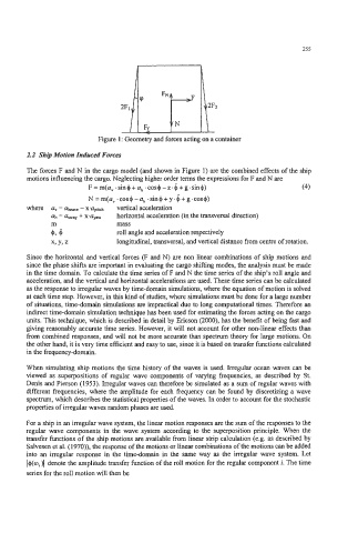
Figure 1 : Geometry and forces acting on a container
2.2 Ship Motion Induced Forces

The forces F and N in the cargo model (and shown in Figure, 1) are the combined effects of the ship
motions influencing the cargo. Neglecting higher order terms the expressions for F and N are
F = m(u, -sin+ + ah .cos+ - z.4 + g -sin+) (4)
N = m(a, . cos+ -ah . sine + y .* + g +cos$)
where a, = akaw - X'upitch vertical acceleration
+
ah = asway xu,, horizontal acceleration (in the transversal direction)
m mass
+, m roll angle and acceleration respectively
x, Y, z longitudinal, transversal, and vertical distance from centre of rotation.
Since the horizontal and vertical forces (F and N) are non linear combinations of ship motions and
since the phase shifts are important in evaluating the cargo shiffig modes, the analysis must be made
in the time domain. To calculate the time series of F and N the time series of the ship's roll angle and
acceleration, and the vertical and horizontal accelerations are used. These time series can be calculated
as the response to irregular waves by time-domain simulations, where the equation of motion is solved
at each time step. However, in this kind of studies, where simulations must be done for a large number
of situations, time-domain simulations are impractical due to long computational times. Therefore an
indirect time-domain simulation technique has been used for estimating the forces acting on the cargo
units. This technique, which is described in detail by Ericson (2000), has the benefit of being fast and
giving reasonably accurate time series. However, it will not account for other non-linear effects than
from combined responses, and will not be more accurate than spectrum theory for large motions. On
the other hand, it is very time efficient and easy to use, since it is based on transfer functions calculated
in the frequency-domain.

When simulating ship motions the time history of the waves is used. Irregular ocean waves can be
viewed as superpositions of regular wave components of varying frequencies, as described by St.
Denis and Pierson (1 953). Irregular waves can therefore be simulated as a sum of regular waves with
different frequencies, where the amplitude for each frequency can be found by discretizing a wave
spectrum, which describes the statistical properties of the waves. In order to account for the stochastic
properties of irregular waves random phases are used.

For a ship in an irregular wave system, the linear motion responses are the sum of the responses to the
regular wave components in the wave system according to the superposition principle. When the
transfer functions of the ship motions are available from linear strip calculation (e.g. as described by
Salvesen et al. (1970)), the response of the motions or linear combinations of the motions can be added
into an irregular response in the time-domain in the same way as the irregular wave system. Let
>I
]+(ai denote the amplitude transfer function of the roll motion for the regular component i. The time
series for the roll motion will then be