Page 302 - Practical Design Ships and Floating Structures

211

1975). The variance o2 represents the total energy of the sea state and is computed as the area
contained in the design spectrum.

Observations of sea states (all directions) Distribution of sea state observations
%class in [SI 7000
H,-dass 5.0 7 0 9 0 11.0 13.0 15.0 17.0 19 0 21.0 23.0 total number of obsewations
in [m]
- 5.0 7 0 9.0 11.0 13.0 15.0 17 0 19.0 21.0 6000 31224=[100%1
- - - -
- - - -
0.0
- -
12.0-150 0 0 0 1 1 0 0 0 0 0 20
11.0-12.0 0 0 0 1 2 0 0 0 0 0
9.5-11.0 0 0 0 1 0 0 0 I 0 0
9 0- 9.5 2 8 26 32 47 23 12 3 0 0 - 5wo
85-90 0 4 7 25 15 7 3 0 0 0 s
8.0- 6.5 0 1 15 13 21 13 4 0 0 0 0 .- 15
7.5- 6.0 2 10 31 35 40 26 9 2 0 3
70-75 1 18 45 41 30 14 7 3 0 0 U
6.5- 7.0 5 21 35 34 31 18 8 1 0 0 f 4000
6 0- 6.5 6 40 66 103 71 24 13 2 0 3 n 0
5.5- 6.0 3 34 97 120 76 33 15 3 0 2 2 3000 10
5 0- 5.5 0 21 79 65 56 24 5 1 0 1 0 n
m
4.5- 5.0 3 34 71 80 25 14 2 0 1 1 E
4 0- 4.5 25 193 421 397 241 69 28 17 I 0 2 2000 ? n
3.5- 4.0 25 204 480 411 195 58 28 7 2 1
3 0- 3.5 48 435 769 555 253 75 13 5 0 0 5
2 5- 3.0 98 681 1015 504 224 46 13 10 2 0
2.0- 2.5 229 1325 1455 620 185 65 13 6 1 2 1MxI
1 5- 2.0 478 2049 1460 368 119 30 10 3 0 0
1 .O- 1.5 1565 2660 1083 275 65 35 13 6 3 4
0.5- 1.0 2600 1448 321 123 42 6 3 6 5 48 0 0
0.2- 0.5 1558 I79 46 20 8 6 4 6 5 63
0 0- 0.2 514 24 18 11 4 0 2 1 7 4 0 30 60 90 120 150 180210240270300330
Nom East South West
sum of Observations rp = 33146 direction of wave ongin p [degrees]
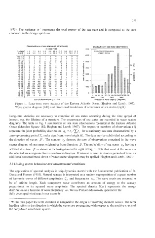
Figure 1. Long-term wave statistic of the Eastern Atlantic Ocean (Hogben and Lumb, 1967).
Wave scatter diagram (left) and directional breakdown of occurrence of sea states (right).
Long-term statistics are necessary to comprise all sea states occurring during the time spread of
interest, e.g. the lifetime of a structure. The occurrences of sea states are recorded in wave scatter
diagrams. The table in Fig. 1 summarizes all sea state observations recorded at the Eastern Atlantic
Ocean (Marsden Square 182; Hogben and Lumb, 1967). The respective numbers of observations r ij
represent the joint probability distribution q,, = r,, /cy,, for a stationary sea state characterized by a
zero-up-crossing period T,,, and a significant wave height H,,. The data may be subdivided according to
the direction of waves PI. The number rp denotes the sum of observations contained in the wave
scatter diagram of sea states originating from direction p . The probability of sea states qp having a
selected direction p is shown in the histogram on the right of Fig. 1. Note that most of the waves in
the selected area originate from a southwest direction. If interest is taken in shorter periods of time, an
additional seasonal break-down of wave scatter diagrams may be applied (Hogben and Lumb, 1967). ’
2.3 Linking system behaviour and environmental conditions
The application of spectral analysis in ship dynamics started with the fundamental publication of St.
Denis and Pierson (1953). Natural seaway is interpreted as a random superposition of a great number
of harmonic waves of different amplitudes <,, and frequencies w, . The wave crests are assumed to
be of infinite length. Each component wave contributes an amount of energy to the seaway
proportional to its squared wave amplitude. The spectral density S(w) represents the energy
distribution as a function of wave frequency w . We use Pierson-Moskowitz spectra for the
fully developed wind seas in our example.
Within this paper the term direction is assigned to the origin of incoming incident waves. The term
heading refers to the direction in which the waves are propagating with respect to the positive x-axis of
the body-fixed coordinate system.