Page 378 - Practical Design Ships and Floating Structures

353

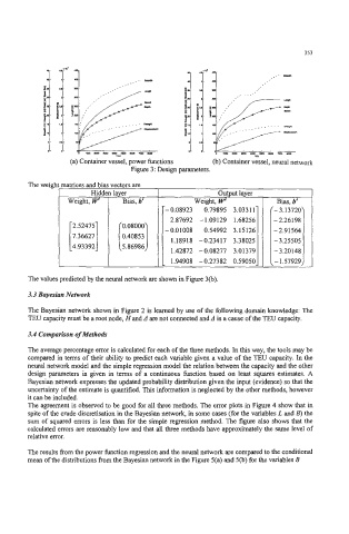
(a) Container vessel, power functions (b) Container vessel, neural network
Figure 3: Design parameters.
The weigl natrices and bias vectors are
Hiddc layer Output layer
Weight, W' Bias, b' 1 Weight, FV Bias, bz
-.
r- 0.08923 0.79895 3.0331 1 - 3.13720
2.87692 -1.09129 1.68256 -2.26198
2.52475
-0.01008 0.54992 3.15126 - 2.91 564
b.366271 1.18918 -0.23417 3.38025 -3.25505
4.93392
1.42872 -0.08277 3.01379 - 3.20148
1.94908 - 0.27382 0.59050 - 1.57929
L
The values predicted by the neural network are shown in Figure 3@).

3.3 Bayesian Network

The Bayesian network shown in Figure 2 is learned by use of the following domain knowledge: The
TEU capacity must be a root node, Hand A are not connected and A is a cause of the TEU capacity.
3.4 Comparison of Methods

The average percentage error is calculated for each of the three methods. In this way, the tools may be
compared in terms of their ability to predict each variable given a value of the TEU capacity. In the
neural network model and the simple regression model the relation between the capacity and the other
design parameters is given in terms of a continuous function based on least squares estimates. A
Bayesian network expresses the updated probability distribution given the input (evidence) so that the
uncertainty of the estimate is quantified. This infomation is neglected by the other methods, however
it can be included.
The agreement is observed to be good for all three methods. The error plots in Figure 4 show that in
spite of the crude discretisation in the Bayesian network, in some cases (for the variables L and B) the
sum of squared errors is less than for the simple regression method. The figure also shows that the
calculated errors are reasonably low and that all three methods have approximately the same level of
relative error.
The results from the power function regression and the neural network are compared to the conditional
mean of the distributions from the Bayesian network in the Figure 5(a) and 5(b) for the variables B