Page 377 - Practical Design Ships and Floating Structures

352

discretised for equal number of ships in each interval. This approach has the characteristic that the
dense part of the distribution is finely discretised so that the variable is well represented in these
regions, whereas the sparse regions are represented by fewer and longer intervals. A pattern search
algorithm is applied to optimise the locations of the discretising split-points, so that the categories
become as uniform as possible. Each variable is discretised into 12 intervals, which is a rather crude,
but to obtain reliable probability estimates, a reasonable number of data points in each interval is
necessary.

Learning a Bayesian network is a task of constructing the network topology and estimating the
associated probability tables, so that the underlying discretised data set is represented in the best
possible way. In this study, the BNPC-algorithm by Cheng, Bell and Liu (2000) is used. Once the
‘optimal’ topology is found, the conditional) probabilities associated with each node are estimated.

3 SINGLE INPUT REGRESSIONS
In the following, the methods just described are used to predict the main particulars of container
vessels. when the prediction is made on the basis of just one input parameter, this must in some sense
be the governing one, in this case TEU capacity. Relations are found for length, L, breadth, B, velocity,
V, draught, D, depth, H, and displacement, A.

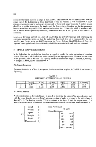
3.1 SimpIe Regression
Expressed in the form of Eqn. 1, the power functions are fitted as given in TABLE 1 and shown in
Figure 3(a).

TABLE 1
COEFFICIENTS OF FITTED POWER LAW FUNCTIONS

a I 8.79 1 3.1

3.2 NeuraI Network

A network structure as shown in Figure 1 is used. It is found that the output of the network agrees well
with the given data (i.e. no over-fitting) when the number of nodes or neurons in the hidden layer is
three (s‘ = 3). The loading capacity (TEU) is assigned to the input P, and the output vector, T, is
ordered as shown below. Also shown are the normalisation matrices for the input P and the output T.
Length L1
Breadth B
Speed V
T= 69.2 347.0
Draught D 13.3 42.8
Depth H 10.0 26.3
Displacement A -
3.0 14.5
5.0 24.4
- 295.5 142800 -