Page 472 - Practical Design Ships and Floating Structures

447

3 DISCRETIZATION AND SINGULARITY DISTRIBUTION
-.
To solve the integral equation for a(X,), the collocation method is used. Field points are chosen
along the real boundary and sources are distributed outside the computational domain. A set of field
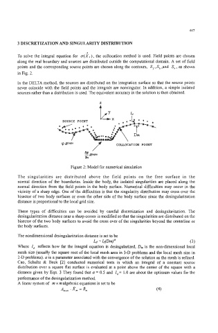
points and the corresponding source points are chosen along the contours, S, , S, ,and S, , as shown
in Fig. 2.

In the DELTA method, the sources are distributed on the integration surface so that the source points
never coincide with the field points and the integrals are nonsingular. In addition, a simple isolated
sources rather than a distribution is used. The equivalent accuracy in the solution is then obtained.

SOURCE POINT

Dm

cp given

Figure 2: Model for numerical simulation
The singularities are distributed above the field points on the free surface in the
normal direction of the boundaries. Inside the body, the isolated singularities are placed along the
normal direction from the field points in the body surface. Numerical difficulties may occur in the
vicinity of a sharp edge. One of the difficulties is that the singularity distribution may cross over the
bisector of two body surfaces or even the other side of the body surface since the desingularization
distance is proportional to the locaI grid size.
These types of difficulties can be avoided by careful discretization and desingularization. The
desingularization distance near a sharp comer is modified so that the singularities are distributed on the
bisector of the two body surfaces to avoid the cross over of the singularities beyond the centerline or
the body surfaces.

The nondimensional desingularization distance is set to be
Ld = IdDm)= (3)
Where I, reflects how far the integral equation is desingularized, Dm is the non-dimensional local
mesh size (usually the square root of the local mesh area in 3-D problems and the local mesh size in
2-D problems). a is a parameter associated with the convergence of the solution as the mesh is refined.
Cao, Schultz & Beck [2] conducted numerical tests in which an integral of a constant source
distribution over a square flat surface is evaluated at a point above the center of the square with a
distance given by Eqn. 3 They found that a = 0.5 and I, = 1 .O are about the optimum values for the
performance of the desingularization method.
A linear system of m x rnalgebraic equations is set to be
-
-
Amxm Xm = Bm (4)