Page 235 - Practical Ship Design

Powering II I97

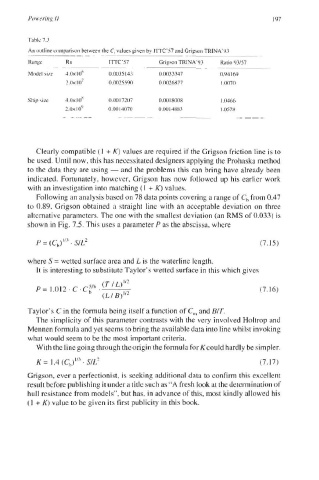
Table 7.3
4n outline comparison between the C, value5 given by ITTC’57 and Grigson TRINA’93
- -~
~~~~~~~~ ~~
Range Rn ITTC’57 Grigson TRINA’93 Ratio 93/57
~~ ~~
~~ ~
Model we 4 0x10’ 00035143 0 0033347 0 94169
2 ox I 0’ 0 0025590 0 0026877 I 0070
Ship \i~e 4 0x1Ox 0 00 17207 0.001 8008 1 0466
2 OX1O9 0 00 14070 0 0014883 1 0578
~ ~ ~~ ~~~~ ~ ~~~~

Clearly compatible (1 + K) values are required if the Grigson friction line is to
be used. Until now, this has necessitated designers applying the Prohaska method
to the data they are using - and the problems this can bring have already been
indicated. Fortunately, however, Grigson has now followed up his earlier work
with an investigation into matching (1 + K) values.
Following an analysis based on 78 data points covering a range of C, from 0.47
to 0.89, Grigson obtained a straight line with an acceptable deviation on three
alternative parameters. The one with the smallest deviation (an RMS of 0.033) is
shown in Fig. 7.5. This uses a parameter P as the abscissa, where

P = ( Cb) ‘I3 ’ S1L2 (7.15)

where S = wetted surface area and L is the waterline length.
It is interesting to substitute Taylor’s wetted surface in this which gives

(7.16)

Taylor’s C in the formula being itself a function of C, and BIT.
The simplicity of this parameter contrasts with the very involved Holtrop and
Mennen formula and yet seems to bring the available data into line whilst invoking
what would seem to be the most important criteria.
With the line going through the origin the formula for K could hardly be simpler.

K = 1.4 (Cb)I13 . SIL’ (7.17)
Grigson, ever a perfectionist, is seeking additional data to confirm this excellent
result before publishing it under a title such as “A fresh look at the determination of
hull resistance from models”, but has, in advance of this, most kindly allowed his
(1 + K) value to be given its first publicity in this book.