Page 240 - Practical Ship Design

202 Chapter 7

figures at the lowest F,, figures were in many cases higher than those quoted for the
next three F, values. It is uncertain whether this came about because of experi-
mental error, noting that such low speed data was of little interest at the time these
tests were made, or because the data was cross faired for presentation purposes. It
was for this reason that this data was not used for a Prohaska analysis of (1 + K)
described in 57.1.2.
After a lot of thought the author came to the conclusion that the only plot that
would avoid all these pitfalls is one of C,, - and that this would have the further
advantage that it can equally well be used for calculations based on the Grigson
friction line and (1 + K) formula described in 57.1.3 which is probably the most
accurate powering method currently available.
To standardise the C,, plots, these have all been based on a model length of 5 m
and have an LIB ratio of 7.28 and a TIL ratio of 0.06.
The fact that the lines are plotted for odd Froude numbers is because these
numbers equate exactly with the VI& values used in the original presentations and
this avoids introducing inaccuracy from the cross fairinghnterpolation necessary if
the curves were to be drawn at single digit Froude numbers - and at the end of a
designer’s calculations the answer will in any case be a powerhpeed plot.
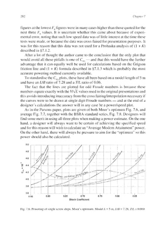
As in the Parsons paper, plots are given of both Moor’s optimum Fig. 7.6, and
average Fig. 7.7, together with the BSRA standard series, Fig. 7.8. Designers will
find some merit in using all three plots when making a power estimate. On the one
hand, a designer will always want to be certain of achieving the specified speed
and for this reason will wish to calculate an “Average Modern Attainment” power.
On the other hand, there will always be pressure to aim for the “optimum” so this
power should also be calculated.

Fig. 7.6. Powering of single screw ships. Moor’s optimum. Model L = 5 m, LIB = 7.28, TIL = 0.060.