Page 337 - Pressure Swing Adsorption

I,
314 PRESSURE SWING ADSORPTION APPENDIX B
315
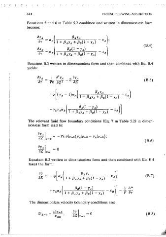
Equations 5 and 6 m Table 5.2 combined and written in dimens1onlcss form The clean bed mmal conditions given by Eq. 12 111 Tahle 5.2 assume the
become: following dimensionless form:

YA(z,0) = 0; y (z,O) = O;
8
(B.9)
xA(z,O) = O; x (z,0) = 0
(B.4) 8

Eauatmn B.3 written in dimens1oniess form and then combined with Eo. B.4
yields: B.2 Collocation Form of the Dimensmnless LDF
Model Equations

(B.5)
When Ea. B.5 with the boundary conditions given by Ea. B.6 ace wntten m
the coIIocation form based on a Legendre-type polynomial to represent the
trial function, the following set of ordinary differential equatmns is obtained:

d M+l
::u) = L [PmBx(j,i) -V(i)Ax(j,i)]YA(i) (B.10)
!..,.2

-A,[Pm Bx(,, 1) - v(j)Ax(j, l)]
The reievant fluid flow boundary conditions (Eq. 7 m Table 5.2) in dimen- M+J
s10ntess form lead to: X L [A 3 Ax(M + 2,i) - Ax(l,i)[YA(i)
,-z

+A 1 [PmBx(J,M+ 2) -v(j)Ax( ,M+ 2)]
1
(B.6)
M+l
X L lA,Ax(M+ 2,i) -Ax(l,i)'JyA(i)
!=2
Equation B.2 wntten in dimensionless form and then combined with Ea. 8.4 M+,
takes the form: -A 4[Pm Bx(}, I) - V(j)Ax(j, I)] L Ax( M + 2, i)yA(i)
•=2
(B.7) +A,[PmBx(i, 1) -D(j)Ax(;, l)]PeD(l)yAlz-11-
-A,[Pm Bx(j, M + 2) - v(j)Ax(j, M + 2)]Pe D(l)yAlz-11-

The dimensionless velocity boundary conditions are:
_ vlz-o av\
V 1 Z=O = --, - =0 (B.8)
VOl-t az z-1
J = 2, ... , M + l