Page 55 - Pressure Swing Adsorption

,.

30
PRESSURE SWING AOSOHl'TION FUNDAMENTALS OF AIJSOl!PTION 31
I b I disadvantage that Ii 1s essenua!ly an cmpmc:.d data fit with iitlle t!1eoretica1
basis.

10
r 2.or-~~~~__, 2.2.9 Ideal Adsorbed Soiution Theory 15
~ ~
~ na
~ . . ....
.§. 10 ...... A more soohist1cated wav of predicting binary and mult1comoonent equilibna
~ from smgle•component isotherms is the ideal al1Sorbcd solution theory. For a
~ 0,6 .;; smgie•componenl system the rclat1onshin between: !-ipreading pressure and
E
/"d'
r::r 0.-4 loading can be found directly by integration of the Gibbs isotherm (Eq. 2.12):
0.6
-,,.A - JP/" 01 ) do (2.16)
'9 RT - q, 'P P
.P o 3031< ()
f 6 29)K
o~-~-~-~-~-~ + 2761< where A is now expressed on a molar IJas,s. The Gibbs isotherm for a binary
0 2 6 8 10 svstem may be wntten as:
P (Bori 04 06
x,, Ad-rr
RT = q A d In PA + l/ B cl In Pn (2.17)
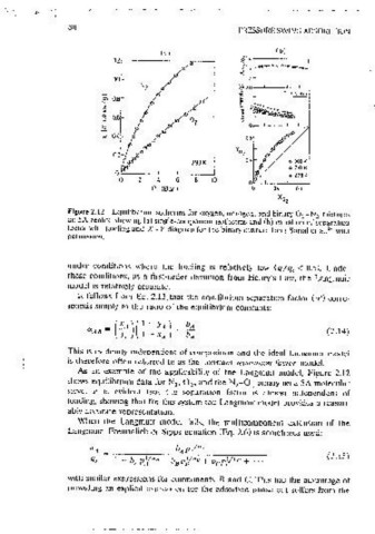
Figure 2.12 Equilibrium isotherms for oxygen, nitrogen, and binary O..,-N mixtures
2 or, at constant total pressure (P):
on 5A zeolite showmg (a) smgie~componeni isotherms and (b) vanat10~ of separation
factor with loading and X -Y diagram for the binary nuxrure from Sona! et ai. 24 with A d-,r
perm1ss1on. (2.18)
RT =qAdlny_. 1 +qndlny 11
where Yi 1s the mole fraction II1 the vapor phase.
If the adsorbed phase 1s thermodynam1cally ideal. the parual pressure p
under conditions where the loading 1s relatively iow (q/q, < 0.5). Under 1
at a specified spreading pressure ( rr) 1s given by:
these conditwns, as a firstMorder deviation from Henry;s Law, the Langmulf
model ts reiat1ve1y accurate. (2.19)
lt follows from Ea. 2.13 that the equilibrium separatmn factor (a') correM
where X; 1s the moie fraction m the adsorbed phase and pf is the vapor
soonds simply to the ratio of the eauilibrium constants:
pressure for the srngle-comoonent system at the same spreading pressure,
calculated from Eq. 2.16. In the mixture the spreading pressure must be the
(2.14) same for both components for a binary system; so we have the followmg set
of equat10ns:
This 1s cvidcntiy independent of composition und the ideal Langmuir modci
0 I ( ") = 11 11 PJJ "
1s therefore often referred to as the constant separatwn factor model. 7TA = l'IA PA I ( ") = 7T/I
As an example of the applicability of the Langrnu1r model, Figure 2.12
PA= PyA = p~XA
shows equilibrmm data for N , 0 , and the N -O binary on a SA moiecular
2 2 2 2
sieve. lt 1s evident that the scnarat\On factor 1s aimost mdcocndcnl of Pn = Pyu = pj:x 11
loading, showmg that for this system the Langmmr model provides a reason- YA :_yB= J.0
ably accurate representation. +
xA=x 8 =1.0 ( 2.20)
When the Langmuir model fails, the mult1comoonent extens10n of the
Langmuir-Freundlich or Sipps eauation (Eq. 2.6) 1s sometimes used: This 1s a set of seven equations relating the nine vanables (X.4. x 8 , v .. •
1
YB, P, 1r:I, 1r~, P,~, p;!); so with anv two variables (e .. g., P and yA) specified
one may calculaic all other vanab\es.
(2.15)
The total concentration m the adsorhed ohase 1s given by:
with s1miiar expressions for comoonents B and C. This has the advantage of ( 2.21)
providing an explicit expression for the adsorbed phase but suffers from the qtot