Page 204 - Probability and Statistical Inference

4. Functions of Random Variables and Sampling Distribution 181

respectively with parameters (n + n , p) and (n , p). Next, one may use
2
1
3
mathematical induction to claim that is thus distributed as the Bino-
mial ( ). !
4.2.2 Continuous Cases

The distribution function approach works well in the case of continuous ran-
dom variables. Suppose that X is a continuous real valued random variable
and let Y be a real valued function of X. The basic idea is first to express the
distribution function G(y) = P(Y ≤ y) of Y in the form of the probability of an
appropriate event defined through the original random variable X. Once the
expression of G(y) is found in a closed form, one would obviously obtain
dG(y)/dy, whenever G(y) is differentiable, as the pdf of the transformed ran-
dom variable Y in the appropriate domain space for y. This technique is ex-
plained with examples.
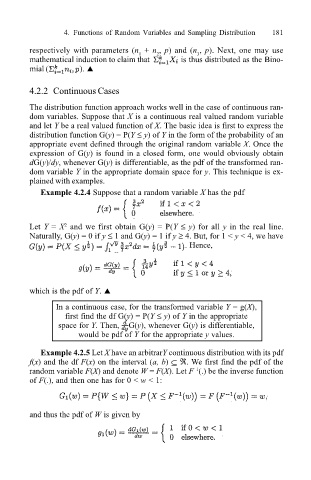
Example 4.2.4 Suppose that a random variable X has the pdf

Let Y = X and we first obtain G(y) = P(Y ≤ y) for all y in the real line.
2
Naturally, G(y) = 0 if y ≤ 1 and G(y) = 1 if y ≥ 4. But, for 1 < y < 4, we have
. Hence,

which is the pdf of Y. !

In a continuous case, for the transformed variable Y = g(X),
first find the df G(y) = P(Y ≤ y) of Y in the appropriate
space for Y. Then, G(y), whenever G(y) is differentiable,
would be pdf of Y for the appropriate y values.

Example 4.2.5 Let X have an arbitrarY continuous distribution with its pdf
f(x) and the df F(x) on the interval (a, b) ⊆ ℜ. We first find the pdf of the
–1
random variable F(X) and denote W = F(X). Let F (.) be the inverse function
of F(.), and then one has for 0 < w < 1:

and thus the pdf of W is given by