Page 203 - Probability and Statistical Inference

180 4. Functions of Random Variables and Sampling Distribution

X values: –1 0 2 2.5
2
Probabilities: .1 .2 .4 .3
Now, P(X = x ∩ X = x ) = P(X = x )P(X = x ) for all X = 0, 1, 3 and X =
1
1
2
1
2
1
2
1
2
2
–1, 0, 2, 2. 5. Suppose that we want to obtain the pmf for the random variable
Y = X + X . The possible values Y of Y belong to the set γ = {–1, 0, 1, 2, 2.5,
1
2
3, 3.5, 5, 5.5}. Now P(Y = 0) = P(X = 0 ∩ X = 0) + P(X = 1 ∩ X = –1) =
1
1
2
2
1 ∩ X = –1) = (.2)(.2) + (.3)(.1) = .07. Also, P(Y = 2) = P(X = 0 ∩ X = 2)
1
2
2
+ P(X = 3 ∩ X = –1) = (.2)(.4) + (.5)(.1) = .13, and this way the pmf
1 2
function g(y) = P(Y = y) can be obtained for all y ∈ y. "
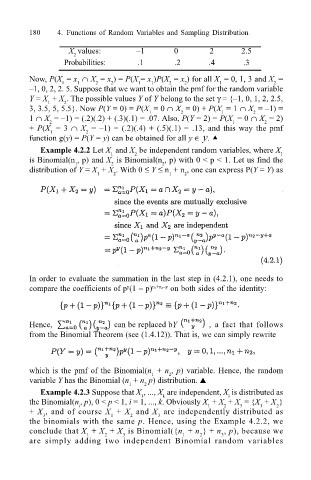
Example 4.2.2 Let X and X be independent random variables, where X 1
1
2
is Binomial(n , p) and X is Binomial(n , p) with 0 < p < 1. Let us find the
2
2
1
distribution of Y = X + X . With 0 ≤ Y ≤ n + n , one can express P(Y = Y) as
1 2 1 2
In order to evaluate the summation in the last step in (4.2.1), one needs to
compare the coefficients of p (1 – p) n 1 +n 2 –y on both sides of the identity:
y
Hence, can be replaced bY , a fact that follows
from the Binomial Theorem (see (1.4.12)). That is, we can simply rewrite

which is the pmf of the Binomial(n + n , p) variable. Hence, the random
1
2
variable Y has the Binomial (n + n p) distribution. !
1 2
Example 4.2.3 Suppose that X , ..., X are independent, X is distributed as
k
i
1
the Binomial(n , p), 0 < p < 1, i = 1, ..., k. Obviously X + X + X = {X + X }
2
2
1
1
i
3
+ X , and of course X + X and X are independently distributed as
3
1
2
3
the binomials with the same p. Hence, using the Example 4.2.2, we
conclude that X + X + X is Binomial({n + n } + n , p), because we
2
3
1
1
2
3
are simply adding two independent Binomial random variables