Page 202 - Probability and Statistical Inference

4. Functions of Random Variables and Sampling Distribution 179

freedom. Thus the pdf of W is given by g(w) = 1/2exp{–1/2ω}I(ω > 0).
Refer to Section 1.7 as needed. The required probability, P(W ≤ a) is simply
then

which matches with the answer found earlier in (4.1.3). This second ap-
proach appears much simpler. !
In the Exercise 4.1.1, we have proposed a direct approach to evaluate
,with some fixed but arbitrary b > 0, where Z , Z are iid stan-
1
2
dard normal. The Exercise 4.5.4, however, provides an easier way to evaluate
the same probability by considering the sampling distribution of the random
variable Z /Z which just happens (Exercise 4.5.1 (iii)) to have the Cauchy
1
2
distribution defined in (1.7.31). The three Exercises 4.5.7-4.5.9 also fall in the
same category.
4.2 Using Distribution Functions

Suppose that we have independent random variables X , ..., X and let us
n
1
denote Y = g (X , ..., X ), a real valued function of these random variables.
1
n
Our goal is to derive the distribution of Y.
If X , ..., X or Y happen to be discrete random variables, we set out to
n
1
evaluate the expression of P(Y = y) for all appropriate y ∈ y, and then by
identifying the form of P(Y = y), we are often led to one of the standard
distributions.
In the continuous case, the present method consists of first obtaining the
distribution function of the new random variable Y, denoted by F(y) = P(Y ≤
y) for all appropriate values of y ∈ y. If F(y) is a differentiable function of Y,
then by differentiating F(y) with respect to y, one can obtain the pdf of Y at
the point y. In what follows, we discuss the discrete and continuous cases
separately.

4.2.1 Discrete Cases

Here we show how some discrete situations can be handled. The exact tech-
niques used may vary from one problem to another.
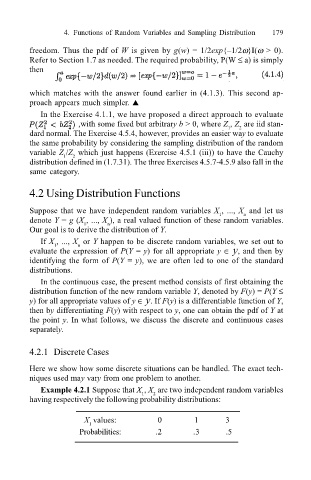
Example 4.2.1 Suppose that X , X are two independent random variables
2
1
having respectively the following probability distributions:
X values: 0 1 3
1
Probabilities: .2 .3 .5