Page 283 - Probability and Statistical Inference

260 5. Concepts of Stochastic Convergence

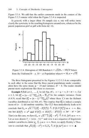
Figure 5.3.4. We add that the earlier comments made in the context of the
Figure 5.3.3 remain valid when the Figure 5.3.4 is inspected.
In general, with a larger (than 10) sample size n, one will notice more
clearly the symmetry in the resulting histograms around zero, whatever be the
parent population pmf or pdf with finite σ(> 0).

Figure 5.3.4. Histogram of 100 Random Values
from the Uniform(10 – a, 10 + a) Population when

The three histograms presented in the Figures 5.3.2-5.3.4 are comparable
to each other in the sense that the three parent populations under consider-
ation have the same mean, µ = 10 and variance, σ = 4. The reader should
2
pursue more explorations like these as exercises.
Example 5.3.6 Let X , ..., X be iid N(µ, σ ), –∞ < µ < ∞, 0 < σ < ∞. For
2
1 n
n ≥ 2, let be the sample variance. From
(4.4.9), recall that where these Y ’s are the Helmert
i
variables distributed as iid N(0, σ ). This implies that is indeed a sample
2
mean of (n – 1) iid random variables. The CLT then immediately leads us to
conclude that as n → ∞. But,
4
one has 3σ – σ = 2σ .
4
4
That is in this case, we have N (0, 2σ ) as n → ∞.
4
Let us now denote V = {n/(n – 1)} and view it as a sequence of degenerate
1/2
n
random variables to claim: as n → ∞. Next, we apply Slutsky’s Theo-
rem to conclude that as n → ∞. !