Page 282 - Probability and Statistical Inference

5. Concepts of Stochastic Convergence 259

the histogram of the 100 randomly observed values of the standardized sample
mean, namely, , ..., 100. The Figure 5.3.2 shows
the histogram which gives an impression of a standard normal pdf.

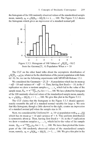
Figure 5.3.3. Histogram of 100 Values of -10)/2
from the Gamma(25, .4) Population When n = 10

The CLT on the other hand talks about the asymptotic distribution of
, whatever be the distribution of the parent population with finite
σ(> 0). So, we ran the following experiments with MINITAB Release 12.1.
We considered the Gamma(α = 25, β = .4) population which has its mean µ
= αβ = 10 and variance σ = αβ = 4. Then, having first fixed n = 10, in the i th
2
2
replication we drew n random samples x , ..., x which led to the value of the
1i ni
sample mean, for i = 1,..., 100. We have plotted the histogram
of the 100 randomly observed values of the standardized sample mean, namely,
, i = 1, ..., 100. We give this plot in the Figure 5.3.3.
The CLT claims that the histogram in the Figure 5.3.3 should approxi-
mately resemble the pdf of a standard normal variable for large n. We note
that this histogram, though a little skewed to the right, creates an impression
of a standard normal pdf when the sample size is 10.
Next, we considered the Uniform(10 – a, 10+a) population with
2
which has its mean µ = 10 and variance σ = 4. This uniform distribution
th
is symmetric about µ. Then, having first fixed n = 10, in the i replication
we drew n random samples x , ..., x which led to the value of the sample
1i ni
mean, for i = 1, ..., 100. We have then plotted the histo-
gram of the 100 randomly observed values of the standardized sample
mean, namely, , i = 1, ..., 100. We give this plot in the