Page 277 - Probability and Statistical Inference

254 5. Concepts of Stochastic Convergence

It is clear that all points u ∈ (–∞, 0) ∪ (0, ∞) are continuity points of the
function F(u), and for all such u, . F (u)=F(u)Hence, we would say that
n
as n → ∞.Hence, asymptotically U has the standard exponential
n
distribution, that is the Gamma(1,1) distribution.!

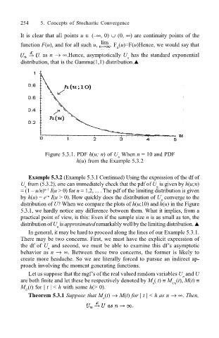
Figure 5.3.1. PDF h(u; n) of U When n = 10 and PDF
n
h(u) from the Example 5.3.2

Example 5.3.2 (Example 5.3.1 Continued) Using the expression of the df of
U from (5.3.2), one can immediately check that the pdf of U is given by h(u;n)
n
n
= (1 – u/n) I(u > 0) for n = 1,2, ... . The pdf of the limiting distribution is given
n–1
by h(u) = e I(u > 0). How quickly does the distribution of U converge to the
–u
n
distribution of U? When we compare the plots of h(u;10) and h(u) in the Figure
5.3.1, we hardly notice any difference between them. What it implies, from a
practical point of view, is this: Even if the sample size n is as small as ten, the
distribution of U is approximated remarkably well by the limiting distribution. !
n
In general, it may be hard to proceed along the lines of our Example 5.3.1.
There may be two concerns. First, we must have the explicit expression of
the df of U and second, we must be able to examine this df’s asymptotic
n
behavior as n → ∞. Between these two concerns, the former is likely to
create more headache. So we are literally forced to pursue an indirect ap-
proach involving the moment generating functions.
Let us suppose that the mgf’s of the real valued random variables U and U
n
are both finite and let these be respectively denoted by M ( t) ≡ M (t), M(t) ≡
Un
n
M (t) for | t | < h with some h(> 0).
U
Theorem 5.3.1 Suppose that M (t) → M(t) for | t | < h as n → ∞. Then,
n