Page 278 - Probability and Statistical Inference

5. Concepts of Stochastic Convergence 255

A proof of this result is beyond the scope of this book. One may refer to
Serfling (1980) or Sen and Singer (1993).
The point is that once M(t) is found, it must correspond to a unique ran-
dom variable, say, U. In the Section 2.4, we had talked about identifying a
distribution uniquely (Theorem 2.4.1) with the help of a finite mgf. We can
use the same result here too.
Also, one may recall that the mgf of the sum of n independent random
variables is same as the product of the n individual mgf’s (Theorem 4.3.1).
This result was successfully exploited earlier in the Section 4.3. In the follow-
ing example and elsewhere, we will repeatedly exploit the form of the mgf of
a linear function of iid random variables all over again.

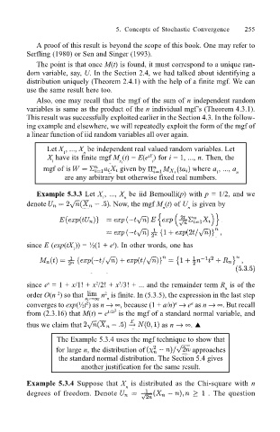
Let X , ..., X be independent real valued random variables. Let
n
1
X have its finite mgf M (t) = E(e ) for i = 1, ..., n. Then, the
tX
i x i i
mgf of is given by where a , ..., a n
1
are any arbitrary but otherwise fixed real numbers.
Example 5.3.3 Let X , ..., X be iid Bernoulli(p) with p = 1/2, and we
1 n
denote . Now, the mgf M (t) of U is given by
n n

since E (exp(tX )) = ½(1 + e ). In other words, one has
t
1

since e = 1 + x/1! + x /2! + x /3! + ... and the remainder term R is of the
3
2
x
n
2
order O(n ) so that n is finite. In (5.3.5), the expression in the last step
–2
n
n
converges to exp(½t ) as n → ∞, because (1 + a/n) → e as n → ∞. But recall
2
a
from (2.3.16) that M(t) = e 1/2t 2 is the mgf of a standard normal variable, and
thus we claim that as n → ∞. !
The Example 5.3.4 uses the mgf technique to show that
for large n, the distribution of approaches
the standard normal distribution. The Section 5.4 gives
another justification for the same result.
Example 5.3.4 Suppose that X is distributed as the Chi-square with n
n
degrees of freedom. Denote . The question