Page 467 - Probability and Statistical Inference

444 9. Confidence Interval Estimation

9.2.1 Inversion of a Test Procedure

In general, for testing a null hypothesis H : θ = θ against the alternative
0
0
hypothesis H : θ > θ (or H : θ < θ or H : θ ≠ θ ), we look at the subset of
1
1
1
0
0
0
c
the sample space R which corresponds to the acceptance of H . In Chapter
0
8, we had called the subset R the critical or the rejection region. The subset
R which corresponds to accepting H may be referred to as the acceptance
c
0
region. The construction of a confidence interval and its confidence coeffi-
c
cient are both closely tied in with the nature of the acceptance region R and
the level of the test.
Example 9.2.1 (Example 8.4.1 Continued) Suppose that X , ..., X are iid
n
1
+
N(µ, σ ) with the unknown parameter µ ∈ ℜ. We assume that σ ∈ ℜ is
2
known. With preassigned α ∈ (0, 1), the UMP level a test for H : µ = µ 0
0
versus H : µ > µ where µ is a fixed real number, would be as follows:
0
1
0
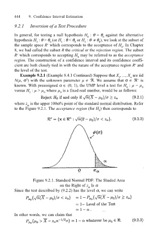
where z is the upper 100α% point of the standard normal distribution. Refer
α
to the Figure 9.2.1. The acceptance region (for H ) then corresponds to
0

Figure 9.2.1. Standard Normal PDF: The Shaded Area
on the Right of z Is α
α
Since the test described by (9.2.2) has the level α, we can write

In other words, we can claim that