Page 469 - Probability and Statistical Inference

446 9. Confidence Interval Estimation

In other words, we can claim that

The equation (9.2.7) can be rewritten as

and thus we can claim that lower
confidence interval estimator for θ. !
Example 9.2.3 (Example 9.2.2 Continued) Let X , ..., X be iid with the
n
1
–1
common exponential pdf θ exp{ –x/θ}I(x > 0) with the unknown parameter
θ ∈ ℜ . With preassigned α ∈ (0,1), suppose that we invert the UMP level α
+
test for H : θ = θ versus H : θ < θ , where θ is a positive real number.
0
0
0
1
0

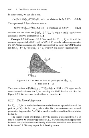
Figure 9.2.3. The Area on the Left (or Right) of ,
1– α Is a (or 1 – α)

Then, one arrives at a 100(1 – α)% upper confi-
dence interval estimator for θ, by inverting the UMP level α test. See the
Figure 9.2.3. We leave out the details as an exercise. !

9.2.2 The Pivotal Approach

Let X , ..., X be iid real valued random variables from a population with the
n
1
pmf or pdf f(x; θ) for x ∈ χ where θ(∈ Θ) is an unknown real valued
parameter. Suppose that T ≡ T(X) is a real valued (minimal) sufficient statis-
tic for θ.
The family of pmf or pdf induced by the statistic T is denoted by g(t; θ)
for t ∈ T and θ ∈ Θ. In many applications, g(t; θ) will belong to an appropriate
location, scale, or location–scale family of distributions which were discussed
in Section 6.5.1. We may expect the following results: