Page 472 - Probability and Statistical Inference

9. Confidence Interval Estimation 449

+
σ ∈ ℜ is known. Given some α ∈ (0,1), we wish to construct a (1 – α) two-
sided confidence interval for µ. The statistic T = , the sample mean, is
2
minimal sufficient for µ and T has the N(µ, 1/nσ ) distribution which belongs
to the location family. The pivot U = has the standard normal
distribution. See the Figure 9.2.4. We have P{ –z < U < z } = 1 – α which
α/2
α/2
implies that

In other words,

is a (1 – α) two–sided confidence interval estimator for µ. !
Example 9.2.8 Normal Mean with Unknown Variance: Suppose that
X , ..., X are iid N(µ, α ) with both unknown parameters µ ∈ ℜ and σ ∈
2
1
n
+
ℜ , n ≥ 2. Given some α ∈ (0,1), we wish to construct a (1 – α) two-
sided confidence interval for µ. Let be the sample mean and
be the sample variance. The statistic T ≡
( , S) is minimal sufficient for (µ, σ). Here, the distributions of the X’s
belong to the location–scale family. The pivot has the
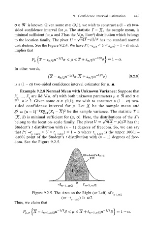
Student’s t distribution with (n – 1) degrees of freedom. So, we can say
that P{ –t n–1,α/2 < U < t n–1,α/2 } = 1 – α where t n–1,α/2 is the upper 100(1 –
½α)% point of the Student’s t distribution with (n – 1) degrees of free-
dom. See the Figure 9.2.5.

Figure 9.2.5. The Area on the Right (or Left) of t n–1,α/2
(or –t n–1,α/2 ) Is α/2
Thus, we claim that