Page 476 - Probability and Statistical Inference

9. Confidence Interval Estimation 453

interval with the same coverage probability (1 – α), then we should have
instead mimicked that in order to arrive at the proposed confidence inter-
vals.
Let us focus on the Example 9.2.7 and explain the case in point. Suppose
that Z is the standard normal random variable. Now, we have P{–z < Z <
α/2
z } = 1 – α. Suppose that one can determine two other positive numbers a,
α/2
b such that P{–a < Z < b} = 1 – α and at the same time 2z > b + a. That is,
α/2
the two intervals (–z ,z ) and (–a, b) have the same coverage probability
α/2 α/2
(1 – α), but (–a, b) is a shorter interval. In that case, instead of the solution
proposed in (9.2.9), we should have suggested
as the confidence interval for µ. One may ask: Was the solution in (9.2.9)
proposed because the interval (–z ,z ) happened to be the shortest one
α/2
α/2
with (1 – α) coverage in a standard normal distribution? The answer is: yes,
that is so. In the case of the Example 9.2.8, the situation is not quite the same
but it remains similar. This will become clear if one contrasts the two Ex-
amples 9.2.12–9.2.13. For the record, let us prove the Theorem 9.2.1 first.

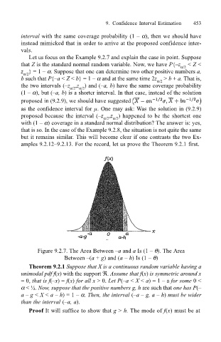
Figure 9.2.7. The Area Between –a and a Is (1 – θ). The Area
Between –(a + g) and (a – h) Is (1 – θ)
Theorem 9.2.1 Suppose that X is a continuous random variable having a
unimodal pdf f(x) with the support ℜ. Assume that f(x) is symmetric around x
= 0, that is f(–x) = f(x) for all x > 0. Let P(–a < X < a) = 1 – a for some 0 <
α < ½. Now, suppose that the positive numbers g, h are such that one has P(–
a – g < X < a – h) = 1 – α. Then, the interval (–a – g, a – h) must be wider
than the interval (–a, a).
Proof It will suffice to show that g > h. The mode of f(x) must be at