Page 481 - Probability and Statistical Inference

458 9. Confidence Interval Estimation

From the Example 4.4.12, recall that 2(n – 1)W /σ is distributed as ,
i
i = 1, 2, and these are independent. Using the reproductive property of inde-
pendent Chi-squares (Theorem 4.3.2, part (iii)) we can claim that 4(n – 1)W σ –
P
1 = {2(n – 1)W + 2(n – 1)W }σ which has a Chi-square distribution with
–1
1
2
4(n – 1) degrees of freedom. Also, and W are independent. Hence,
P
we may use the following pivot
Now, let us look into the distribution of U. We know that

Hence, the pdf of Q = Y – Y would be given by ½e I(q ∈ ℜ) so that the
–|q|
1
2
random variable | Q | has the standard exponential distribution. Refer to the
Exercise 4.3.4, part (ii). In other words, 2| Q | is distributed as . Also Q, W P
are independently distributed. Now, we rewrite the expression from (9.3.5)
as

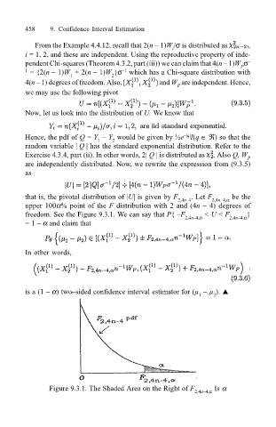
that is, the pivotal distribution of |U| is given by F 2,4n–4 . Let F 2,4n–4,α be the
upper 100α% point of the F distribution with 2 and (4n – 4) degrees of
freedom. See the Figure 9.3.1. We can say that P{ –F 2,4n–4,α < U < F 2,4n–4,α }
= 1 – α and claim that

In other words,

is a (1 – α) two–sided confidence interval estimator for (µ – µ ). !
1 2

Figure 9.3.1. The Shaded Area on the Right of F Is α
2,4n–4,α