Page 477 - Probability and Statistical Inference

454 9. Confidence Interval Estimation

x = 0. We may assume that a > h since we have 0 < α < ½. Since we have
P(–a < X < a) = P(–a – g < X < a – h), one obviously, has

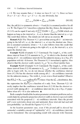
But, the pdf f(x) is symmetric about x = 0 and f(x) is assumed positive for all
x ∈ ℜ. The Figure 9.2.7 describes a situation like this. Hence, the integrals in
(9.2.15) can be equal if and only if which can
happen as long as the interval (a – h, a) is shorter than the interval (a, a +g).
The result then follows. The details are left out as an exercise. !
Remark 9.2.1 The Theorem 9.2.1 proved that among all (1 – α) intervals
going to the left of (–a, a), the interval (–a, a) was the shortest one. Since,
f(x) is assumed symmetric about x = 0, it also follows from this result that
among all (1 – α) intervals going to the right of (–a, a), the interval (–a, a) is
again the shortest one.
Example 9.2.12 (Example 9.2.7 Continued) The length L of the confi-
n
dence interval from (9.2.9) amounts to 2z n σ which is the shortest width
–½
α/2
2
among all (1 – α) confidence intervals for the unknown mean µ in a N(µ, σ )
population with σ(> 0) known. The Theorem 9.2.1 immediately applies. Also
–½
observe that the shortest width, namely 2z n σ, is a fixed number here.
α/2
Example 9.2.13 (Example 9.2.8 Continued) The length L of the confi-
n
–½
dence interval from (9.2.10) amounts to 2t n–1,α/2 n S which is a random vari-
able to begin with. So, we do not discuss whether the confidence interval
from (9.2.10) has the shortest width among all (1 – α) confidence intervals
for the unknown mean µ. The width L is not even a fixed number! Observe
n
that where Y has the distribution. But,
the expression for is a function of n only. Now, Theorem 9.2.1 di-
rectly implies that the confidence interval from (9.2.10) has the shortest ex-
2
pected width among all (1 – a) confidence intervals for µ in a N(µ, s ) popu-
2
lation when σ (> 0) is also unknown. !
Both examples handled the location parameter estimation problems and we
could claim the optimality properties (shortest width or shortest expected width)
associated with the proposed (1 – α) confidence intervals. Since the pivotal
pdf’s were symmetric about zero and unimodal, these intervals had each tail
area probability ½α. Recall the Figures 9.2.4–9.2.5.
In the location parameter case, even if the pivotal pdf is skewed but
unimodal, a suitable concept of “optimality” of (1 – α) confidence intervals
can be formulated. The corresponding result will coincide with Theorem