Page 475 - Probability and Statistical Inference

452 9. Confidence Interval Estimation

keep constructing the corresponding observed confidence interval estimates
(T (x ), T (x )), (T (x ), T (x )), (T (x ), T (x )), .... In the long run, out of
1
U
1
U
3
L
2
L
3
L
2
U
all these intervals constructed, approximately 100(1 – α)% would include the
unknown value of the parameter θ. This goes hand in hand with the relative
frequency interpretation of probability calculations explained in Chapter 1.
In a frequentist paradigm, one does not talk about the probability of a fixed
interval estimate including or not including the unknown value of θ.
Example 9.2.11 (Example 9.2.1 Continued) Suppose that X , ..., X are iid
n
1
N(µ, σ ) with the unknown parameter µ ∈ ℜ. We assume that s ∈ ℜ + is
2
known. We fix α = .05 so that will be a 95% lower
confidence interval for µ. Using the MINITAB Release 12.1, we generated a
normal population with µ = 5 and σ = 1. First, we considered n = 10. In the
th
i replication, we obtained the value of the sample mean and computed the
lower end point of the observed confidence interval, i = 1, ..., k
with k = 100, 200, 500. Then, approximately 5% of the total number (k) of
intervals so constructed can be expected not to include the true value µ = 5.
Next, we repeated the simulated exercise when n = 20. The following table
summarizes the findings.
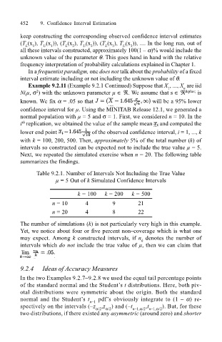
Table 9.2.1. Number of Intervals Not Including the True Value
µ = 5 Out of k Simulated Confidence Intervals
k = 100 k = 200 k = 500
n = 10 4 9 21
n = 20 4 8 22

The number of simulations (k) is not particularly very high in this example.
Yet, we notice about four or five percent non–coverage which is what one
may expect. Among k constructed intervals, if n denotes the number of
k
intervals which do not include the true value of µ, then we can claim that

9.2.4 Ideas of Accuracy Measures

In the two Examples 9.2.7–9.2.8 we used the equal tail percentage points
of the standard normal and the Student’s t distributions. Here, both piv-
otal distributions were symmetric about the origin. Both the standard
normal and the Student’s t n–1 pdf’s obviously integrate to (1 – α) re-
,t
spectively on the intervals (–z α/2 ,z α/2 ) and (–t n–1,α/2 n–1,α/2 ). But, for these
two distributions, if there existed any asymmetric (around zero) and shorter