Page 482 - Probability and Statistical Inference

9. Confidence Interval Estimation 459

Confidence interval estimation of (µ – µ )/σ in the two Examples
2
1
9.3.1-9.3.2 using the Bonferroni inequality are left as Exercises
9.3.3 and 9.3.5. Look at the Example 9.2.10 as needed.
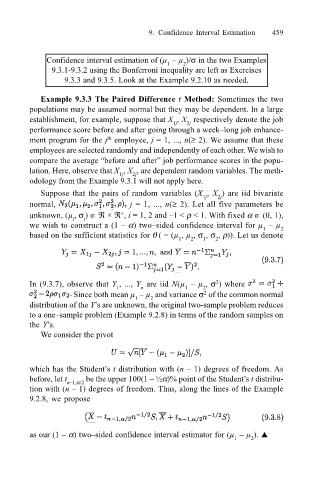
Example 9.3.3 The Paired Difference t Method: Sometimes the two
populations may be assumed normal but they may be dependent. In a large
establishment, for example, suppose that X , X respectively denote the job
2j
1j
performance score before and after going through a week–long job enhance-
th
ment program for the j employee, j = 1, ..., n(≥ 2). We assume that these
employees are selected randomly and independently of each other. We wish to
compare the average “before and after” job performance scores in the popu-
lation. Here, observe that X , X , are dependent random variables. The meth-
1j
2j
odology from the Example 9.3.1 will not apply here.
Suppose that the pairs of random variables (X , X ) are iid bivariate
1j
2j
normal, j = 1, ..., n(≥ 2). Let all five parameters be
+
unknown, (µ , σ ) ∈ ℜ × ℜ , i = 1, 2 and –1 < ρ < 1. With fixed α ∈ (0, 1),
i
i
we wish to construct a (1 – α) two–sided confidence interval for µ – µ 2
1
based on the sufficient statistics for θ ( = (µ , µ , σ , σ , ρ)). Let us denote
1 2 1 2

2
In (9.3.7), observe that Y , ..., Y are iid N(µ – µ , σ ) where
n
1
1
2
Since both mean µ – µ and variance σ of the common normal
2
1
2
distribution of the Y’s are unknown, the original two-sample problem reduces
to a one–sample problem (Example 9.2.8) in terms of the random samples on
the Y’s.
We consider the pivot
which has the Student’s t distribution with (n – 1) degrees of freedom. As
before, let t n–1,α/2 be the upper 100(1 – ½α)% point of the Student’s t distribu-
tion with (n – 1) degrees of freedom. Thus, along the lines of the Example
9.2.8, we propose

as our (1 – α) two–sided confidence interval estimator for (µ – µ ). !
2
1