Page 49 - Probability and Statistical Inference

26 1. Notions of Probability

The expression for F (w) is clear for w ≤ 1 since in this case we inte-
W
grate the zero density. The expression for F (w) is also clear for w ≥ 2
W
because the associated integral can be written as
For 1 < w < 2, the expression for F (w can be
W
written as . It should
be obvious that the df F (w) is continuous at all points
W
w ∈ ℜ but F (w) is not differentiable specifically at the two points w = 1, 2. In
W
this sense, the df F (w) may not be considered very smooth. !
W
The pmf in (1.6.6) gives an example of a discrete random variable
whose df has countably infinite number of discontinuity points. The
pdf in (1.6.9) gives an example of a continuous random variable
whose df is not differentiable at countably infinite number of points.

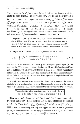
Example 1.6.5 Consider the function f(x) defined as follows:

We leave it as the Exercise 1.6.4 to verify that (i) f(x) is a genuine pdf, (ii) the
associated df F(x) is continuous at all points x ∈ ℜ, and (iii) F(x) is not differ-
entiable at the points x belonging to the set which is countably
infinite. In the Example 1.6.2, we had worked with the point masses at count-
ably infinite number of points. But, note that the present example is little differ-
ent in its construction. !
In each case, observe that the set of the discontinuity points of the associ-
ated df F(.) is at most countably infinite. This is exactly what one will expect in
view of the Theorem 1.6.1. Next, we proceed to calculate probabilities of events.

The probability of an event or a set A is given by the area
under the pdf f(x) wherever f(x) is positive, x ∈ A.

Example 1.6.6 (Example 1.6.4 Continued) For the continuous dis-
tribution defined by (1.6.7), suppose that the set A stands for the interval
(–1.5, 1.8). Then, P(A) = =
. Alternately, we may also apply the form of the df given by
(1.6.8) to evaluate the probability, P(A) as follows: P(A) = P(1 < W < 1.8) =
F (1.8) – F (1) = 1/7{(1.8) – 1} – 0 = . !
3
W W