Page 46 - Probability and Statistical Inference

1. Notions of Probability 23

This is a simple result to prove. We leave its proof as Exercise 1.5.6.

It is true that any function F(x), x ∈ ℜ, which satisfies the
properties (i)-(iii) stated in the Theorem 1.5.1 is in fact a df
of some uniquely determined random variable X.

1.6 Continuous Random Variables

A continuous random variable, commonly denoted by X, Y and so on, takes
values only within subintervals of ℜ or within subsets generated by some ap-
propriate subintervals of the real line ℜ. At a particular location in a lake, for
example, the manager of the local parks and recreation department may be
interested in studying the pattern of the depth (X) of the water level. In a high-
rise office building, for example, one may be interested to investigate the pat-
tern of the waiting time (X) for an elevator on any of its floors. At the time of the
annual music festival in an amusement park, for example, the resident manager
at a nearby senior center may want to study the pattern of the loudness factor
(X). These are some typical examples of continuous random variables.

1.6.1 Probability Density and Distribution Functions

We assume that the sample space S itself is a subinterval of ℜ. Now, a con-
tinuous real valued random variable X is a mapping of S into the real line ℜ. In
this scenario, we no longer talk about P(X = x) because this probability will be
zero regardless of what specific value x ∈ ℜ one has in mind. For example,
the waiting time (X) at a bus stop would often be postulated as a continuous
random variable, and thus the probability of one’s waiting exactly five minutes
or exactly seven minutes at that stop for the next bus to arrive is simply zero.
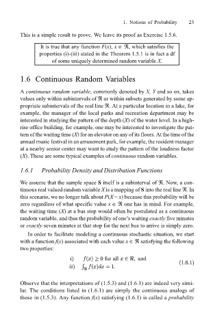
In order to facilitate modeling a continuous stochastic situation, we start
with a function f(x) associated with each value x ∈ ℜ satisfying the following
two properties:

Observe that the interpretations of (1.5.3) and (1.6.1) are indeed very simi-
lar. The conditions listed in (1.6.1) are simply the continuous analogs of
those in (1.5.3). Any function f(x) satisfying (1.6.1) is called a probability