Page 44 - Probability and Statistical Inference

1. Notions of Probability 21

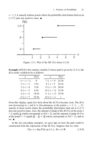
x = 1, 2, 4, namely at those points where the probability distribution laid out in
(1.5.7) puts any positive mass. !

Figure 1.5.1. Plot of the DF F(x) from (1.5.8)

Example 1.5.2 For the random variable X whose pmf is given by (1.5.1), the
df is easily verified to be as follows:
x F(x) x F(x)
–∞ < x < 2 0 7 ≤ x < 8 21/36
2 ≤ x < 3 1/36 8 ≤ x < 9 26/36
3 ≤ x < 4 3/36 9 ≤ x < 10 30/36
4 ≤ x < 5 6/36 10 ≤ x < 11 33/36
5 ≤ x < 6 10/36 11 ≤ x < 12 35/36
6 ≤ x < 7 15/36 12 ≤ x < ∞ 1

From this display, again few facts about the df F(x) become clear. The df is
non-decreasing in x and it is discontinuous at the points x = 2, 3, ..., 12,
namely at those points where the probability distribution laid out in (1.5.1)
puts any positive mass. Also, the amount of jump of the df F(x) at the point x
= 2 equals which corresponds to P(X = 2), and the amount of jump of F(x)
at the point x = 3 equals which corresponds to P(X = 3), and so
on. !
In the two preceding examples, we gave tips on how the pmf could be
constructed from the expression of the df F(x). Suppose that we write