Page 47 - Probability and Statistical Inference

24 1. Notions of Probability

density function (pdf).

A probability mass function (pmf) or probability density function
(pdf) f(x) is respectively defined through (1.5.3) and (1.6.1).

Once the pdf f(x) is specified, we can find the probabilities of various
events defined in terms of the random variable X. If we denote a set A( ⊆ ℜ),
then

where the convention is that we would integrate the function f(x) only on that
part of the set A wherever f(x) is positive.
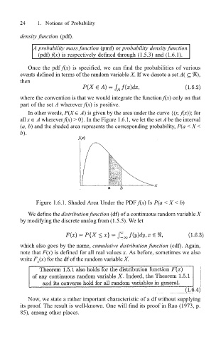
In other words, P(X ∈ A) is given by the area under the curve {(x, f(x)); for
all x ∈ A wherever f(x) > 0}. In the Figure 1.6.1, we let the set A be the interval
(a, b) and the shaded area represents the corresponding probability, P(a < X <
b).

Figure 1.6.1. Shaded Area Under the PDF f(x) Is P(a < X < b)

We define the distribution function (df) of a continuous random variable X
by modifying the discrete analog from (1.5.5). We let

which also goes by the name, cumulative distribution function (cdf). Again,
note that F(x) is defined for all real values x. As before, sometimes we also
write F (x) for the df of the random variable X.
X

Now, we state a rather important characteristic of a df without supplying
its proof. The result is well-known. One will find its proof in Rao (1973, p.
85), among other places.