Page 43 - Probability and Statistical Inference

20 1. Notions of Probability

a discrete distribution or a discrete probability distribution of the random
variable X.

The function f(x) = P(X = x) for x ∈ χ = {x , x , ..., x , ...} is
1
2
i
customarily known as the probability mass function (pmf) of X.
We also define another useful function associated with a random variable
X as follows:

which is customarily called the distribution function (df) or the cumulative
distribution function (cdf) of X. Sometimes we may instead write F (x) for the
X
df of the random variable X.
A distribution function (df) or cumulative distribution function (cdf)
F(x) for the random variable X is defined for all real numbers x

Once the pmf f(x) is given as in case of (1.5.4), one can find the probabili-
ties of events which are defined through the random variable X. If we denote a
set A(⊆ ℜ;), then

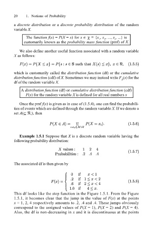
Example 1.5.1 Suppose that X is a discrete random variable having the
following probability distribution:

The associated df is then given by

This df looks like the step function in the Figure 1.5.1. From the Figure
1.5.1, it becomes clear that the jump in the value of F(x) at the points
x = 1, 2, 4 respectively amounts to .2, .4 and .4. These jumps obviously
correspond to the assigned values of P(X = 1), P(X = 2) and P(X = 4).
Also, the df is non-decreasing in x and it is discontinuous at the points