Page 42 - Probability and Statistical Inference

1. Notions of Probability 19

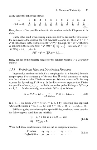
easily verify the following entries:

Here, the set of the possible values for the random variable X happens to be
finite.
On the other hand, when tossing a fair coin, let Y be the number of tosses of
the coin required to observe the first head (H) to come up. Then, P(Y = 1) =
P(The H appears in the first toss itself) = P(H) = 1/2, and P(Y = 2) = P(The first
1
1
1
H appears in the second toss) = P(TH) = ( ( ( ( = ( ( Similarly, P(Y = 3) =
2 2 4
P(TTH) = 1/8, ..., that is
Here, the set of the possible values for the random variable Y is countably
infinite.

1.5.1 Probability Mass and Distribution Functions
In general, a random variable X is a mapping (that is, a function) from the
sample space S to a subset χ of the real line ℜ which amounts to saying
that the random variable X induces events (∈ ß) in the context of S. We may
express this by writing X : S → χ. In the discrete case, suppose that X takes
the possible values x , x , x , ... with the respective probabilities p = P(X = x ),
2
3
i
i
1
i = 1, 2, ... . Mathematically, we evaluate P(X = x ) as follows:
i
In (1.5.1), we found P(X = i) for i = 2, 3, 4 by following this approach
whereas the space χ ={2, 3, ..., 12} and S = {11, ..., 16, 21, ..., 61, ..., 66}.
While assigning or evaluating these probabilities, one has to make sure that
the following two conditions are satisfied:

When both these conditions are met, we call an assignment such as