Page 515 - Probability and Statistical Inference

492 10. Bayesian Methods

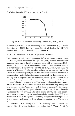
Θ*(b) is going to be 95% when we choose b ≈ .2.

Figure 10.5.1. Plot of the Probability Content q(b) from (10.5.9)

With the help of MAPLE, we numerically solved the equation q(b) = .95 and
found that b ≈ .20077. In other words, (10.5.8) will lead to the HPD 95%
credible interval for v which is (.27812, .72188). !
10.5.2 Contrasting with the Confidence Intervals

Now, we emphasize important conceptual differences in the notions of a 100
(1–α)% confidence interval and a 100(1–α)% (HPD) credible interval for an
unknown parameter . In either case, one starts with an appropriate likeli-
hood function. In the case of a confidence interval, the unknown parameter
is assumed fixed. In the case of a credible interval, however, the unknown
parameter is assumed to be a random variable having some pdf h(θ) on Θ.
Under the frequentist paradigm, we talk about the unknown parameter
belonging to a constructed confidence interval, only from the point of view of
limiting relative frequency idea. Recall the interpretation given in Section 9.2.3.
On the other hand, under the Bayesian paradigm we can evaluate the poste-
rior probability that v belongs to a credible interval by integrating the posterior
pdf on the interval. In this sense, the confidence coefficient may be regarded
as a measure of initial accuracy which is fixed in advance by the experi-
menter whereas the posterior probability content of a credible interval may be
regarded as the final accuracy. The latter conclusion may look more appeal-
ing in some applications but we may also remind the reader that a HPD cred-
ible interval arises at the expense of assuming that (i) the unknown parameter
is a random variable and (ii) has a known prior distribution h(α) for α ∈
Θ.
Example 10.5.5 (Example 10.5.2 Continued) With the sample of
size n = 20 midterm examination scores, we had and σ = 30. So
2