Page 520 - Probability and Statistical Inference

10. Bayesian Methods 497

this with the fact that p(x) is increasing in x(∈ ℜ) to validate (10.7.7). In other
words, the expression of is always positive. Also refer to the Exercises
10.7.2-10.7.3. !
In the three previous examples, we had worked with the normal likelihood
function given = θ. But, we were told that v was positive and hence we
were forced to put a prior only on (0, ∞). We experimented with the exponen-
tial prior for which happened to be skewed to the right. In the case of a
normal likelihood, some situations may instead call for a non-conjugate but
symmetric prior for . Look at the next example.
Example 10.7.4 Let X be N(θ, 1) given that = θ where (∈ ℜ) is the
unknown population mean. Consider the statistic T = X which is minimal
sufficient for θ given that = θ. We have been told that (i) is an arbitrary
real number, (ii) is likely to be distributed symmetrically around zero, and
(iii) the prior probability around zero is little more than what it is likely with a
normal prior. With the N(0, 1) prior on , we note that the prior probability of
–3
the interval (–.01, .01) amounts to 7.9787 × 10 whereas with the Laplace
prior pdf h(θ) = ½e I(θ ∈ ℜ), the prior probability of the same interval
–|θ|
amounts to 9.9502 × 10 . So, let us start with the Laplace prior h(θ) for .
–3
From the apriori description of alone, it does not follow however that the
chosen prior distribution is the only viable candidate. But, let us begin some
preliminary investigation anyway.
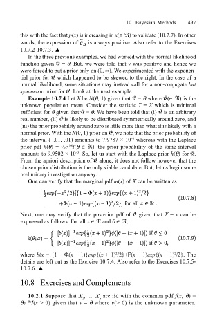
One can verify that the marginal pdf m(x) of X can be written as

Next, one may verify that the posterior pdf of given that X = x can be
expressed as follows: For all x ∈ ℜ and θ ∈ ℜ,

where b(x = {1 – Φ(x + 1)}exp{(x + 1) /2}+F(x – 1)exp{(x – 1) /2}. The
2
2
details are left out as the Exercise 10.7.4. Also refer to the Exercises 10.7.5-
10.7.6. !
10.8 Exercises and Complements

10.2.1 Suppose that X , ..., X are iid with the common pdf f(x; θ) =
1
n
θe I(x > 0) given that v = θ where v(> 0) is the unknown parameter.
–θx