Page 519 - Probability and Statistical Inference

496 10. Bayesian Methods

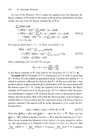
In view of the Theorem 10.4.2, under the squared error loss function, the
Bayes estimate of would be the mean of the posterior distribution. In other
words, one can write the Bayes estimate of as

It is easy to check that I = x – α. Next, we rewrite I as
2 1

Now, combining (10.7.4)-(10.7.5), we get

as the Bayes estimate of . Also refer to the Exercises 10.7.2-10.7.3. !
Example 10.7.3 (Example 10.7.2 Continued) Let X be N(θ, 1) given that
= θ where is the unknown population mean. Consider the statistic T = X
which is minimal sufficient for θ given that = θ. We were told that v was
positive and we supposed that the prior distribution of was exponential with
the known mean α (> 0). Under the squared error loss function, the Bayes
–1
estimate of turned out to be given by (10.7.6). Observe that the poste-
rior distribution’s support is ℜ and thus the mean of this posterior distri-
+
bution, must be positive. But, notice that the observed data x may be larger or
smaller than α. Can we check that the expression of will always lead to a
positive estimate? The answer will be in the affirmative if we verify the fol-
lowing claim:

Note that Φ(x) = φ(x) and φ(x) = –xφ(x) for all x ∈ ℜ. Thus, one has
p(x) = Φ(x) which is positive for all x ∈ ℜ so that the function p(x) ↑ in x.
Next, let us consider the behavior of p(x) when x is near negative infin-
ity. By appealing to L’Hôpital’s rule from (1.6.29), we observe that
Hence, Combine