Page 57 - Probability and Statistical Inference

34 1. Notions of Probability

Refer to the Binomial Theorem from (1.4.12). Next let us look at some ex-
amples.
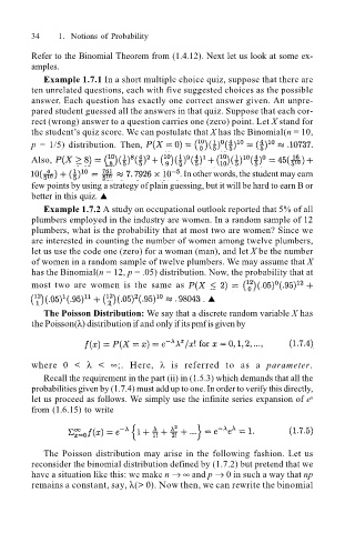
Example 1.7.1 In a short multiple choice quiz, suppose that there are
ten unrelated questions, each with five suggested choices as the possible
answer. Each question has exactly one correct answer given. An unpre-
pared student guessed all the answers in that quiz. Suppose that each cor-
rect (wrong) answer to a question carries one (zero) point. Let X stand for
the student’s quiz score. We can postulate that X has the Binomial(n = 10,
p = 1/5) distribution. Then,
Also,
. In other words, the student may earn
few points by using a strategy of plain guessing, but it will be hard to earn B or
better in this quiz. !
Example 1.7.2 A study on occupational outlook reported that 5% of all
plumbers employed in the industry are women. In a random sample of 12
plumbers, what is the probability that at most two are women? Since we
are interested in counting the number of women among twelve plumbers,
let us use the code one (zero) for a woman (man), and let X be the number
of women in a random sample of twelve plumbers. We may assume that X
has the Binomial(n = 12, p = .05) distribution. Now, the probability that at
most two are women is the same as
. !
The Poisson Distribution: We say that a discrete random variable X has
the Poisson(λ) distribution if and only if its pmf is given by

where 0 < λ < ∞;. Here, λ is referred to as a parameter.
Recall the requirement in the part (ii) in (1.5.3) which demands that all the
probabilities given by (1.7.4) must add up to one. In order to verify this directly,
let us proceed as follows. We simply use the infinite series expansion of e x
from (1.6.15) to write

The Poisson distribution may arise in the following fashion. Let us
reconsider the binomial distribution defined by (1.7.2) but pretend that we
have a situation like this: we make n → ∞ and p → 0 in such a way that np
remains a constant, say, λ(> 0). Now then, we can rewrite the binomial