Page 58 - Probability and Statistical Inference

1. Notions of Probability 35

probability for any fixed x = 0, 1, 2, ... ,

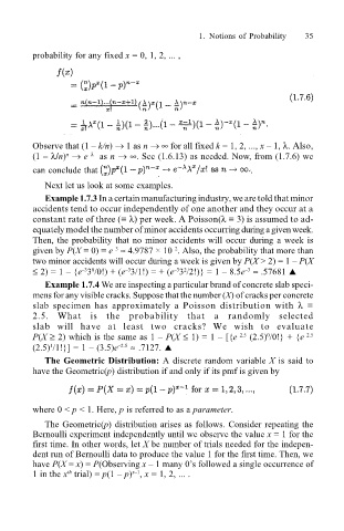
Observe that (1 – k/n) → 1 as n → ∞ for all fixed k = 1, 2, ..., x – 1, λ. Also,
–λ
n
(1 – λ/n) → e as n → ∞. See (1.6.13) as needed. Now, from (1.7.6) we
can conclude that .
Next let us look at some examples.
Example 1.7.3 In a certain manufacturing industry, we are told that minor
accidents tend to occur independently of one another and they occur at a
constant rate of three (= λ) per week. A Poisson(λ = 3) is assumed to ad-
equately model the number of minor accidents occurring during a given week.
Then, the probability that no minor accidents will occur during a week is
–2
–3
given by P(X = 0) = e ≈ 4.9787 × 10 . Also, the probability that more than
two minor accidents will occur during a week is given by P(X > 2) = 1 – P(X
–3
–3 0
–3 2
≤ 2) = 1 – {e 3 /0!) + (e 3/1!) = + (e 3 /2!)} = 1 – 8.5e ≈ .57681 !
–3
Example 1.7.4 We are inspecting a particular brand of concrete slab speci-
mens for any visible cracks. Suppose that the number (X) of cracks per concrete
slab specimen has approximately a Poisson distribution with λ =
2.5. What is the probability that a randomly selected
slab will have at least two cracks? We wish to evaluate
P(X ≥ 2) which is the same as 1 – P(X ≤ 1) = 1 – [{e –2.5 (2.5) /0!} + {e –2.5
0
(2.5) /1!}] = 1 – (3.5)e –2.5 ≈ .7127. !
1
The Geometric Distribution: A discrete random variable X is said to
have the Geometric(p) distribution if and only if its pmf is given by

where 0 < p < 1. Here, p is referred to as a parameter.
The Geometric(p) distribution arises as follows. Consider repeating the
Bernoulli experiment independently until we observe the value x = 1 for the
first time. In other words, let X be number of trials needed for the indepen-
dent run of Bernoulli data to produce the value 1 for the first time. Then, we
have P(X = x) = P(Observing x – 1 many 0’s followed a single occurrence of
x–1
th
1 in the x trial) = p(1 – p) , x = 1, 2, ... .