Page 63 - Probability and Statistical Inference

40 1. Notions of Probability

This proves (1.7.14). An alternative way to prove the same result using the
polar coordinates has been indicated in the Exercise 1.7.20.
The pdf given by (1.7.13) is symmetric around x = µ, that is we have f(x
– µ) = f(x + µ) for all fixed x ∈ ℜ. In other words, once the curve (x, f(x)) is
plotted, if we pretend to fold the curve around the vertical line x = µ, then the
two sides of the curve will lie exactly on one another. See the Figure 1.7.2.
The Standard Normal Distribution: The normal distribution with µ = 0,
σ = 1 is customarily referred to as the standard normal distribution and the
standard normal random variable is commonly denoted by Z. The standard
normal pdf and the df are respectively denoted by

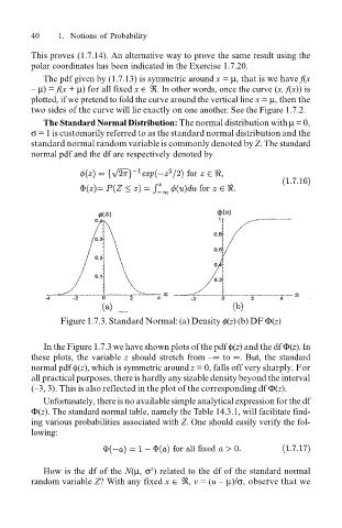
Figure 1.7.3. Standard Normal: (a) Density φ(z) (b) DF Φ(z)

In the Figure 1.7.3 we have shown plots of the pdf φ(z) and the df Φ(z). In
these plots, the variable z should stretch from –∞ to ∞. But, the standard
normal pdf φ(z), which is symmetric around z = 0, falls off very sharply. For
all practical purposes, there is hardly any sizable density beyond the interval
(–3, 3). This is also reflected in the plot of the corresponding df Φ(z).
Unfortunately, there is no available simple analytical expression for the df
Φ(z). The standard normal table, namely the Table 14.3.1, will facilitate find-
ing various probabilities associated with Z. One should easily verify the fol-
lowing:

How is the df of the N(µ, σ ) related to the df of the standard normal
2
random variable Z? With any fixed x ∈ ℜ, v = (u – µ)/σ, observe that we