Page 61 - Probability and Statistical Inference

38 1. Notions of Probability

The Uniform Distribution: A continuous random variable X has the uni-
form distribution on the interval (a, b), denoted by Uniform (a, b), if and only if
its pdf is given by

where –∞ < a, b < ∞. Here, a, b are referred to as parameters.

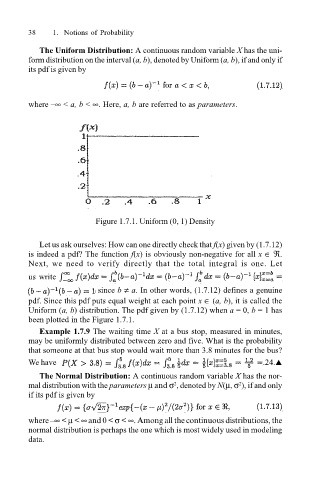
Figure 1.7.1. Uniform (0, 1) Density

Let us ask ourselves: How can one directly check that f(x) given by (1.7.12)
is indeed a pdf? The function f(x) is obviously non-negative for all x ∈ ℜ.
Next, we need to verify directly that the total integral is one. Let
us write
since b ≠ a. In other words, (1.7.12) defines a genuine
pdf. Since this pdf puts equal weight at each point x ∈ (a, b), it is called the
Uniform (a, b) distribution. The pdf given by (1.7.12) when a = 0, b = 1 has
been plotted in the Figure 1.7.1.
Example 1.7.9 The waiting time X at a bus stop, measured in minutes,
may be uniformly distributed between zero and five. What is the probability
that someone at that bus stop would wait more than 3.8 minutes for the bus?
We have .24.!
The Normal Distribution: A continuous random variable X has the nor-
mal distribution with the parameters µ and σ , denoted by N(µ, σ ), if and only
2
2
if its pdf is given by

where –∞ < µ < ∞ and 0 < σ < ∞. Among all the continuous distributions, the
normal distribution is perhaps the one which is most widely used in modeling
data.