Page 64 - Probability and Statistical Inference

1. Notions of Probability 41

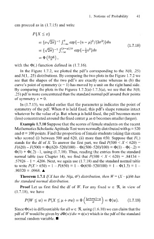
can proceed as in (1.7.15) and write

with the Φ(.) function defined in (1.7.16).
In the Figure 1.7.2, we plotted the pdf’s corresponding to the N(0, .25)
and N(1, .25) distributions. By comparing the two plots in the Figure 1.7.2 we
see that the shapes of the two pdf’s are exactly same whereas in (b) the
curve’s point of symmetry (x = 1) has moved by a unit on the right hand side.
By comparing the plots in the Figures 1.7.2(a)-1.7.3(a), we see that the N(0,
.25) pdf is more concentrated than the standard normal pdf around their points
of symmetry x = 0.
In (1.7.13), we added earlier that the parameter µ indicates the point of
symmetry of the pdf. When σ is held fixed, this pdf’s shape remains intact
whatever be the value of µ. But when µ is held fixed, the pdf becomes more
(less) concentrated around the fixed center µ as σ becomes smaller (larger).
Example 1.7.10 Suppose that the scores of female students on the recent
Mathematics Scholastic Aptitude Test were normally distributed with µ = 520
and σ = 100 points. Find the proportion of female students taking this exam
who scored (i) between 500 and 620, (ii) more than 650. Suppose that F(.)
stands for the df of X. To answer the first part, we find P(500 < X < 620) =
F(620) – F(500) = Φ((620–520)/100) – Φ((500–520)/100) = Φ(1) – Φ(–.2) =
Φ(1) + Φ(.2) –1, using (1.7.18). Thus, reading the entries from the standard
normal table (see Chapter 14), we find that P(500 < X < 620) = .84134 +
.57926 – 1 = .4206. Next, we again use (1.7.18) and the standard normal table
to write P(X > 650) = 1 – F(650) = 1 – Φ(650–520/100) = 1 – Φ(1.3) = 1 –
.90320 = .0968. !
Theorem 1.7.1 If X has the N(µ, σ ) distribution, then W = (X – µ)/σ has
2
the standard normal distribution.
Proof Let us first find the df of W. For any fixed w ∈ ℜ, in view of
(1.7.18), we have

Since Φ(w) is differentiable for all w ∈ ℜ, using (1.6.10) we can claim that the
pdf of W would be given by dΦ(w)/dw = φ(w) which is the pdf of the standard
normal random variable. !