Page 69 - Probability and Statistical Inference

46 1. Notions of Probability

role in statistics. It was discovered by W. S. Gosset under the pseudonym
“Student” which was published in 1908. By varying the values of ν, one can
generate interesting shapes for the associated pdf.

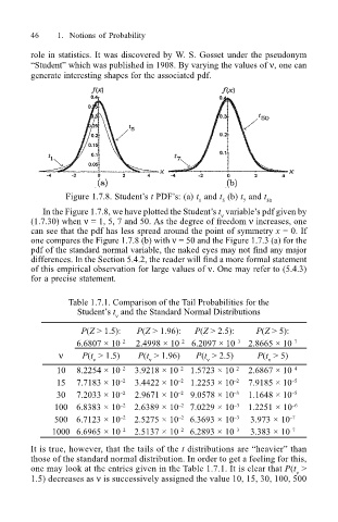
Figure 1.7.8. Student’s t PDF’s: (a) t and t (b) t and t
1 5 7 50
In the Figure 1.7.8, we have plotted the Student’s t variable’s pdf given by
ν
(1.7.30) when ν = 1, 5, 7 and 50. As the degree of freedom ν increases, one
can see that the pdf has less spread around the point of symmetry x = 0. If
one compares the Figure 1.7.8 (b) with ν = 50 and the Figure 1.7.3 (a) for the
pdf of the standard normal variable, the naked eyes may not find any major
differences. In the Section 5.4.2, the reader will find a more formal statement
of this empirical observation for large values of ν. One may refer to (5.4.3)
for a precise statement.

Table 1.7.1. Comparison of the Tail Probabilities for the
Student’s t and the Standard Normal Distributions
ν
P(Z > 1.5): P(Z > 1.96): P(Z > 2.5): P(Z > 5):
6.6807 × 10 –2 2.4998 × 10 –2 6.2097 × 10 –3 2.8665 × 10 –7
ν P(t > 1.5) P(t > 1.96) P(t > 2.5) P(t > 5)
ν
ν
ν
ν
10 8.2254 × 10 –2 3.9218 × 10 –2 1.5723 × 10 –2 2.6867 × 10 –4
15 7.7183 × 10 –2 3.4422 × 10 –2 1.2253 × 10 –2 7.9185 × 10 –5
30 7.2033 × 10 –2 2.9671 × 10 –2 9.0578 × 10 –3 1.1648 × 10 –5
100 6.8383 × 10 –2 2.6389 × 10 –2 7.0229 × 10 –3 1.2251 × 10 –6
500 6.7123 × 10 –2 2.5275 × 10 –2 6.3693 × 10 –3 3.973 × 10 –7
1000 6.6965 × 10 –2 2.5137 × 10 –2 6.2893 × 10 –3 3.383 × 10 –7
It is true, however, that the tails of the t distributions are “heavier” than
those of the standard normal distribution. In order to get a feeling for this,
one may look at the entries given in the Table 1.7.1. It is clear that P(t >
ν
1.5) decreases as ν is successively assigned the value 10, 15, 30, 100, 500