
Page 70 - Probability and Statistical Inference
P. 70
1. Notions of Probability 47
and 1000. Even when ν = 1000, we have P(t > 1.5) = .066965 whereas P(Z
ν
> 1.5) = .066807, that is P(t > 1.5) > P(Z > 1.5). In this sense, the tail of the
ν
t distribution is heavier than that of the standard normal pdf. One may also
ν
note that the discrepancy between P(t > 5) and P(Z > 5) stays large even
ν
when ν = 1000.
The Cauchy Distribution: It corresponds to the pdf of a Students t ν
random variable with ν = 1, denoted by Cauchy(0, 1). In this special case, the
pdf from (1.7.30) simplifies to
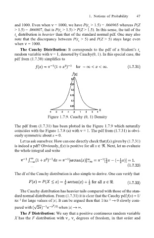
Figure 1.7.9. Cauchy (0, 1) Density
The pdf from (1.7.31) has been plotted in the Figure 1.7.9 which naturally
coincides with the Figure 1.7.8 (a) with ν = 1. The pdf from (1.7.31) is obvi-
ously symmetric about x = 0.
Let us ask ourselves: How can one directly check that f(x) given by (1.7.31)
is indeed a pdf? Obviously, f(x) is positive for all x ∈ ℜ. Next, let us evaluate
the whole integral and write
The df of the Cauchy distribution is also simple to derive. One can verify that
The Cauchy distribution has heavier tails compared with those of the stan-
dard normal distribution. From (1.7.31) it is clear that the Cauchy pdf f(x) ≈ 1/
2
2
πx for large values of |x|. It can be argued then that 1/πx → 0 slowly com-
pared with when |x| → ∞.
The F Distribution: We say that a positive continuous random variable
X has the F distribution with ν , ν degrees of freedom, in that order and
1 2