Page 71 - Probability and Statistical Inference

48 1. Notions of Probability

denoted by F , if and only if its pdf is given by
ν1, ν2

with . Here,
ν and ν are referred to as the parameters. By varying the values of ν and ν ,
2
1
2
1
one can generate interesting shapes for this pdf.

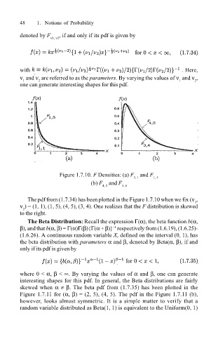
Figure 1.7.10. F Densities: (a) F and F
1, 1 1, 5
(b) F and F
4, 5 3, 4

The pdf from (1.7.34) has been plotted in the Figure 1.7.10 when we fix (ν ,
1
ν ) = (1, 1), (1, 5), (4, 5), (3, 4). One realizes that the F distribution is skewed
2
to the right.
The Beta Distribution: Recall the expression Γ(α), the beta function b(α,
β), and that b(α, β) = Γ(α)Γ(β){Γ(α + β)} respectively from (1.6.19), (1.6.25)-
–1
(1.6.26). A continuous random variable X, defined on the interval (0, 1), has
the beta distribution with parameters α and β, denoted by Beta(α, β), if and
only if its pdf is given by

where 0 < α, β < ∞. By varying the values of α and β, one can generate
interesting shapes for this pdf. In general, the Beta distributions are fairly
skewed when α ≠ β. The beta pdf from (1.7.35) has been plotted in the
Figure 1.7.11 for (α, β) = (2, 5), (4, 5). The pdf in the Figure 1.7.11 (b),
however, looks almost symmetric. It is a simple matter to verify that a
random variable distributed as Beta(1, 1) is equivalent to the Uniform(0, 1)