Page 68 - Probability and Statistical Inference

1. Notions of Probability 45

ν = 25 and 35. In the Section 5.4.1, the reader will find a more formal
statement of this empirical observation for large values of ν. One may refer to
(5.4.2) for a precise statement of the relevant result.
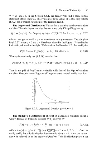
The Lognormal Distribution: We say that a positive continuous random
variable X has the lognormal distribution if and only if its pdf is given by

where – ∞ < µ < ∞ and 0 < σ < ∞ are referred to as parameters. The pdf given
by (1.7.27) when µ = 0 and σ = 1 has been plotted in the Figure 1.7.8 and it also
looks fairly skewed to the right. We leave it as the Exercise 1.7.15 to verify that

We may immediately use (1.7.28) to claim that

That is, the pdf of log(X) must coincide with that of the N(µ, σ ) random
2
variable. Thus, the name “lognormal” appears quite natural in this situation.

Figure 1.7.7. Lognormal Density: µ = 0, σ = 1

The Student’s t Distribution: The pdf of a Student’s t random variable
with ν degrees of freedom, denoted by t , is given by
ν

with ν = 1, 2, 3, ... . One can
easily verify that this distribution is symmetric about x = 0. Here, the param-
eter ν is referred to as the degree of freedom. This distribution plays a key