Page 257 - Process Equipment and Plant Design Principles and Practices by Subhabrata Ray Gargi Das

258 Chapter 10 Absorption and stripping

10.2.1 Graphical determination of the number of contacting stages
Assuming that no chemical reaction occurs and a single component is absorbed from the gas to the
liquid phase, the number of ideal stages is determined from a graphical construction using the oper-
ating and equilibrium curves.
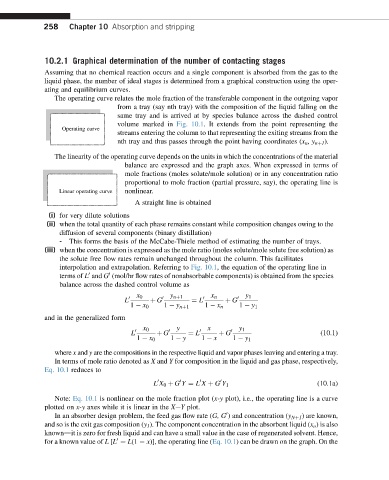
The operating curve relates the mole fraction of the transferable component in the outgoing vapor
from a tray (say nth tray) with the composition of the liquid falling on the
same tray and is arrived at by species balance across the dashed control
volume marked in Fig. 10.1. It extends from the point representing the
Operating curve
streams entering the column to that representing the exiting streams from the
nth tray and thus passes through the point having coordinates (x n , y nþ1 ).

The linearity of the operating curve depends on the units in which the concentrations of the material
balance are expressed and the graph axes. When expressed in terms of
mole fractions (moles solute/mole solution) or in any concentration ratio
proportional to mole fraction (partial pressure, say), the operating line is
Linear operating curve nonlinear.
A straight line is obtained
(i) for very dilute solutions
(ii) when the total quantity of each phase remains constant while composition changes owing to the
diffusion of several components (binary distillation)
- This forms the basis of the McCabe-Thiele method of estimating the number of trays.
(iii) when the concentration is expressed as the mole ratio (moles solute/mole solute free solution) as
the solute free flow rates remain unchanged throughout the column. This facilitates
interpolation and extrapolation. Referring to Fig. 10.1, the equation of the operating line in
terms of L and G (mol/hr flow rates of nonabsorbable components) is obtained from the species
0
0
balance across the dashed control volume as
x 0 y nþ1 x n y 1
L 0 þ G 0 ¼ L 0 þ G 0
1 x 0 1 y nþ1 1 x n 1 y 1
and in the generalized form

x 0 y x y 1
L 0 þ G 0 ¼ L 0 þ G 0 (10.1)
1 x 0 1 y 1 x 1 y 1
where x and y are the compositions in the respective liquid and vapor phases leaving and entering a tray.
In terms of mole ratio denoted as X and Y for composition in the liquid and gas phase, respectively,
Eq. 10.1 reduces to
0 0 0 0 (10.1a)
L X 0 þ G Y ¼ L X þ G Y 1
Note: Eq. 10.1 is nonlinear on the mole fraction plot (x-y plot), i.e., the operating line is a curve
plotted on x-y axes while it is linear in the XeY plot.
In an absorber design problem, the feed gas flow rate (G, G ) and concentration (y Nþ1 ) are known,
0
and so is the exit gas composition (y 1 ). The component concentration in the absorbent liquid (x o ) is also
knowndit is zero for fresh liquid and can have a small value in the case of regenerated solvent. Hence,
for a known value of L [L ¼ L(1 x)], the operating line (Eq. 10.1) can be drawn on the graph. On the
0