Page 258 - Process Equipment and Plant Design Principles and Practices by Subhabrata Ray Gargi Das

10.2 Tray column 259

same graph, the equilibrium solubility data for the solute gas in the solvent liquid can also be plotted in
terms of the same concentration units. Each point on the equilibrium curve represents the gas con-
centration in equilibrium with the liquid at its local concentration and temperature. The position of the
operating line with respect to the equilibrium curve depends on the choice of abscissa and ordinate vis-
a `-vis the direction of mass transfer. The line is above the equilibrium curve if the mass transfer occurs
from gas to liquid phase (absorption), and the composition in the gas phase is represented in the y-axis.
In the case of a stripper, the operating curve is below the equilibrium curve for the same choice of axes.
The number of ideal contacting stages for a design problem can be determined graphically from the
operating and equilibrium curves, as discussed below.

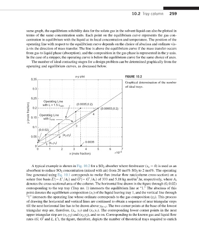
x-y plot FIGURE 10.2
0.35
Graphical determination of the number
of ideal trays.
0.3

0.25
Operating Line (0.0035,0.2)
y (mole fraction) 0.15 Operating Line 4 (0.00503,0.2)
with L = 1.5 L min
0.2
with L
min
0.1 3
(0,0.02)
(x ,y )
0.05 2 2 2
(x 1 ,y ) 0.0035
1
1
0
0 1 2 3 4 5 6 7
x (mole fraction) ×10 –3

A typical example is shown in Fig. 10.2 for a SO 2 absorber where freshwater (x o ¼ 0) is used as an
absorbent to reduce SO 2 concentration (mixed with air) from 20 mol% SO 2 to 2 mol%. The operating
line generated using Eq. 10.1 corresponds to molar flux (molar flow rate/column cross-section) on a
2
0
solute free basis L ð¼ L =A t Þ and G ð¼ G =A t Þ of 333 and 5.18 kg mol/m .hr, respectively, where A t
0
0
0
denotes the cross-sectional area of the column. The horizontal line drawn in the figure through (0, 0.02)
corresponding to the top tray (Tray no. 1) intersects the equilibrium line at “1.” The abscissa of this
point denotes the equilibrium composition (x 1 ) of the liquid leaving tray 1, and the vertical line through
“1” intersects the operating line whose ordinate corresponds to the gas composition (y 2 ). This process
of drawing the horizontal and vertical lines are continued to obtain a sequence of near triangular steps
till the next horizontal line has to be drawn above y Nþ1 . The two corner points at the base of the lowest
triangular step are, therefore, (x o ,y 1 ) and (x 1 ,y 1 ). The corresponding lower corner points in the next
upper triangular step are (x 1 ,y 2 ) and (x 2 ,y 2 ), and so on. Corresponding to the known gas and liquid flow
rates (G, G and L, L ), the figure, therefore, depicts the number of theoretical trays required to enrich
0
0