Page 270 - Process Equipment and Plant Design Principles and Practices by Subhabrata Ray Gargi Das

10.4 Design illustration 271

Usually, the economic use of solvent flow varies from 1.5 to 2.5 times L min . We consider the factor
to be 1.5 times minimum water flow rate. This needs to be verified later.
rL op ¼ 1.5 L min [ 118.71 kmol/hr ¼ 2136.78 kg/hr.
For this flow rate of water, y 1 ¼ 0.1, y 2 ¼ 0.00189, x 2 ¼ 0, x 1 ¼ (6.7 e 0.67) / 118.71 ¼ 0.048.
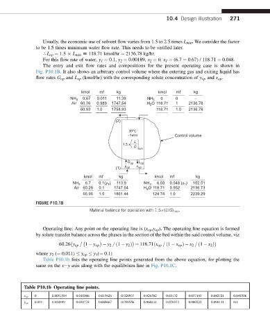
The entry and exit flow rates and compositions for the present operating case is shown in
Fig. P10.1B. It also shows an arbitrary control volume where the entering gas and exiting liquid has
flow rates G op and L op (kmol/hr) with the corresponding solute concentration of y op and x op .

kmol mf kg kmol mf kg
NH 3 0.67 0.011 11.39 NH 3 0 0 –
Air 60.26 0.989 1747.54 H O 118.71 1 2136.78
2
60.93 1.0 1758.93 118.71 1.0 2136.78

(2)
30°C
∼1atm Control volume
L
1.5 x
G
min
G op L op
y x
(1) op op
kmol mf kg kmol mf kg
NH 3 6.7 0.1(y 1 ) 113.9 NH 3 6.03 0.048 (x ) 102.51
1
Air 60.26 0.1 1747.54 H O 118.71 0.952 2136.73
2
66.96 1.0 1861.44 124.74 1.0 2239.29
FIGURE P10.1B
Material balance for operation with 1.5 (L/G) min .

Operating line: Any point on the operating line is (x op ,y op ). The operating line equation is formed
by solute transfer balance across the phases in the section of the bed within the said control volume, viz

60:26 y op = 1 y op y 2 = ð1 y 2 Þ ¼ 118:71ðx op = ð1 x op Þ x 2 = ð1 x 2 ÞÞ
where y 2 (¼ 0.011) y op y 1 (¼ 0.1)
Table P10.1b lists the operating line points generated from the above equation, for plotting the
same on the xey axis along with the equilibrium line in Fig. P10.1C.

Table P10.1b Operating line points.

0 0.0051584 0.010366 0.015626 0.020937 0.026302 0.03172 0.037193 0.042721 0.048306
x op
y op 0.011 0.020889 0.030778 0.040667 0.050556 0.060444 0.070333 0.080222 0.090111 0.1