Page 67 - Process Equipment and Plant Design Principles and Practices by Subhabrata Ray Gargi Das

3.4 Design illustration 63

3.4 Design illustration
3.4.1 Design steps
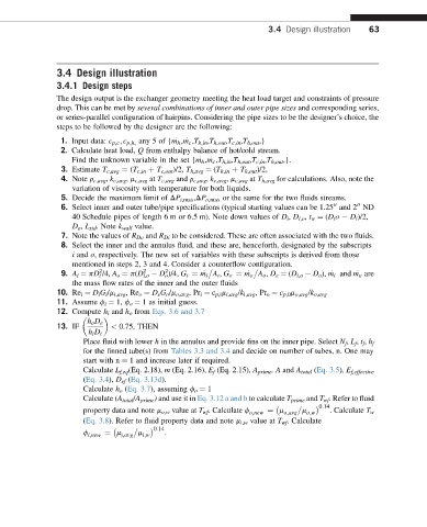
The design output is the exchanger geometry meeting the heat load target and constraints of pressure
drop. This can be met by several combinations of inner and outer pipe sizes and corresponding series,
or series-parallel configuration of hairpins. Considering the pipe sizes to be the designer’s choice, the
steps to be followed by the designer are the following:
: :
1. Input data: c p;c ; c p;h; any 5 of {m h ,m c ,T h,in ,T h,out ,T c,in ,T h,out ,}
2. Calculate heat load, Q from enthalpy balance of hot/cold stream.
: :
Find the unknown variable in the set {m h ,m c ,T h,in ,T h,out ,T c,in ,T h,out ,}.
3. Estimate T c,avg ¼ (T c,in þ T c,out )/2, T h,avg ¼ (T h,in þ T h,out )/2,
4. Note r c,avg , k c,avg , m c,avg at T c,avg and r c,avg , k c,avg , m c,avg at T h,avg for calculations. Also, note the
variation of viscosity with temperature for both liquids.
5. Decide the maximum limit of DP i,max ,DP o,max or the same for the two fluids streams.
6. Select inner and outer tube/pipe specifications (typical starting values can be 1.25 and 2 ND
00
00
40 Schedule pipes of length 6 m or 6.5 m). Note down values of D i , D i,o , t w ¼ (D i o D i )/2,
D o , L std . Note k wall value.
7. Note the values of R Do and R Di to be considered. These are often associated with the two fluids.
8. Select the inner and the annulus fluid, and these are, henceforth, designated by the subscripts
i and o, respectively. The new set of variables with these subscripts is derived from those
mentioned in steps 2, 3 and 4. Consider a counterflow configuration.
:
:
2
2
2
:
:
9. A i ¼ pD i /4, A o ¼ p(D i,o D o )/4, G i ¼ m i A i , G o ¼ m o A o , D e ¼ (D i,o D o ), m i and m o are
the mass flow rates of the inner and the outer fluids
10. Re i ¼ D i G i /m i,avg ,Re o ¼ D e G o /m o,avg ,Pr i ¼ c p,i m i,avg /k i,avg ,Pr o ¼ c p,0 m o,avg /k o,avg
11. Assume f i ¼ 1, f o ¼ 1 as initial guess.
12. Compute h i and h o from Eqs. 3.6 and 3.7

h o D e
13. IF < 0.75, THEN
h i D i
Place fluid with lower h in the annulus and provide fins on the inner pipe. Select N f , L f , t f , h f
for the finned tube(s) from Tables 3.3 and 3.4 and decide on number of tubes, n. One may
start with n ¼ 1 and increase later if required.
Calculate L f,eq (Eq. 2.18), m (Eq. 2.16), E f (Eq. 2.15), A prime ,A and A total (Eq. 3.5),E f,effective
(Eq. 3.4), D ef (Eq. 3.13d).
Calculate h o (Eq. 3.7), assuming f o ¼ 1
Calculate (A total /A prime ) and use it in Eq. 3.12 a and b to calculate T prime and T wf . Refer to fluid
0:14

property data and note m o,w value at T wf . Calculate f o;new ¼ m o;avg m o;w . Calculate T w
(Eq. 3.8). Refer to fluid property data and note m i,w value at T wf . Calculate
0:14

f i;new ¼ m i;avg m i;w .